03 Max Subarray Sum

Lecture from: 03.10.2024 | Video: Videos ETHZ | Rui Zhangs Notes | Leetcode: 53. Maximum Subarray

Max Subarray Sum

Imagine you’re given a list of daily stock price changes. Your goal is to determine the maximum profit you could make by buying and selling the stock at most once. This problem, known as the Max Subarray Sum problem, involves finding the subarray with the largest sum, representing the period where your investment yields the highest return.

Algorithm 0: The Naive Approach ($\Theta (n^3)$)

A simple solution is to consider every possible subarray:

Pseudocode:

def max_subarray_sum_naive(array):
  max_sum = 0
  for i in range(len(array)):
    for j in range(i, len(array)):
      current_sum = 0
      for k in range(i, j):
        current_sum += array[k]
      max_sum = max(max_sum, current_sum)
  return max_sum

Here, we use three nested loops. The outer loop iterates through starting points (i), the second loop through ending points (j), and the innermost loop calculates the sum for each subarray. While this approach is conceptually straightforward, it suffers from a time complexity of $\Theta (n^3)$ due to the triple nesting.

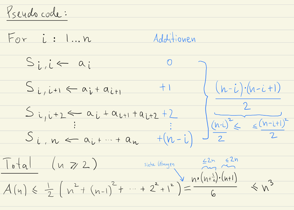
Algorithm 1: Reduce Duplicate Work ($\Theta (n^2)$)

When calculating the sum of a subarray from index i to j, we only need the current element (array[j]) plus the sum of the previous subarray (from index i to j-1). This means we can avoid recalculating the entire subarray sum for each iteration.

Pseudocode:

def max_subarray_sum(array):
  max_sum = 0
  for i in range(len(array)):
    current_sum = 0
    for j in range(i, len(array)):
      current_sum += array[j]  # Add the current element
      max_sum = max(max_sum, current_sum)  # Update max_sum if needed
  return max_sum

Explanation:

1. Initialization: max_sum is initialized to negative infinity to ensure that any valid subarray sum will be greater.
2. Outer Loop (i): This loop iterates through each element as a potential starting point for a subarray.
3. Inner Loop (j): This loop extends the subarray from index i to the current position j.
   • current_sum is updated by adding the value at array[j].
   • We compare current_sum with max_sum and update max_sum if current_sum is larger.

Time Complexity:

The nested loops result in $\Theta (n^2)$ time complexity because the inner loop iterates n-i times for each iteration of the outer loop.

In this current algorithm we are calculating all the possible subarray sums. If we want to improve the time complexity of this algorithm, we need to start thinking how to not need to calculate all the subarray sums (since we can’t reduce the operations more while also calculating all the sums).

Algorithm 3: Divide and Conquer ($\Theta (n\log n)$)

This algorithm leverages the concept of divide and conquer to efficiently solve the Max Subarray Sum problem.

Steps

1. Split: Divide the input array (array) into two roughly equal halves: left_half and right_half.

2. Base Case: If either half contains only one element, its sum is the maximum subarray sum for that half.

3. Recurse:

   • Find the maximum subarray sum (max_left) within left_half recursively.
   • Find the maximum subarray sum (max_right) within right_half recursively.

4. Combine:

   • Calculate the cross_sum: The sum of a subarray spanning both halves. Find the maximum cross_sum by considering all possible starting points in left_half and ending points in right_half.
   • The overall maximum subarray sum (max_sum) is the largest among:
     • max_left (maximum subarray sum in the left half)
     • max_right (maximum subarray sum in the right half)
     • cross_sum (maximum subarray sum spanning both halves)

5. Return: Return max_sum.

Calculating cross_sum

The maximum sum subarray spanning both halves (cross_sum) can be broken down into two parts:

$i\le \frac{n}{2}<j\to max(S_{i,j})=max\left(S_{i,\frac{n}{2}}\right)+max(S_{\frac{n}{2}+1,j})$

To calculate this efficiently, we can adapt the idea from Algorithm 2. Instead of iterating through all possible pairs (i, j), we fix one pointer (either i or j) and incrementally move the other.

For each fixed position, we calculate the maximum subarray sum by:

• Starting from that fixed point.
• Iteratively moving the free pointer and adding its value to the running sum.
• Updating the maximum sum encountered during this process.

This will give us $\frac{n}{2}-1$ additions for each half which means that in total we need $2\left(\frac{n}{2}-1\right)+1=n-1$ additions to find the cross_sum.

Pseudocode:

def max_subarray_sum(array):
  if len(array) == 1:
    return array[0] # Base Case: Single element
 
  midpoint = len(array) // 2
  left_half = array[:midpoint]
  right_half = array[midpoint:]
 
  max_left = max_subarray_sum(left_half)
  max_right = max_subarray_sum(right_half)
  cross_sum = calculate_cross_sum(left_half, right_half)
 
  return max(max_left, max_right, cross_sum) # Overall maximum
 
def calculate_cross_sum(left_half, right_half):
  left_max = current_sum = 0
  for i in range(len(left_half), -1): # Iterate from midpoint backwards
    current_sum += left_half[i]
    left_max = max(left_max, current_sum)
 
  right_max = current_sum = 0
  for j in range(len(right_half)):
    current_sum += right_half[j]
    right_max = max(right_max, current_sum)
 
  cross_sum = left_max + right_max
  return cross_sum

Time Complexity $\Theta (n\log n)$

We can write down the recurrence of additions in the following manner:

$$A(n)=2A\left(\frac{n}{2}\right)+n-1$$

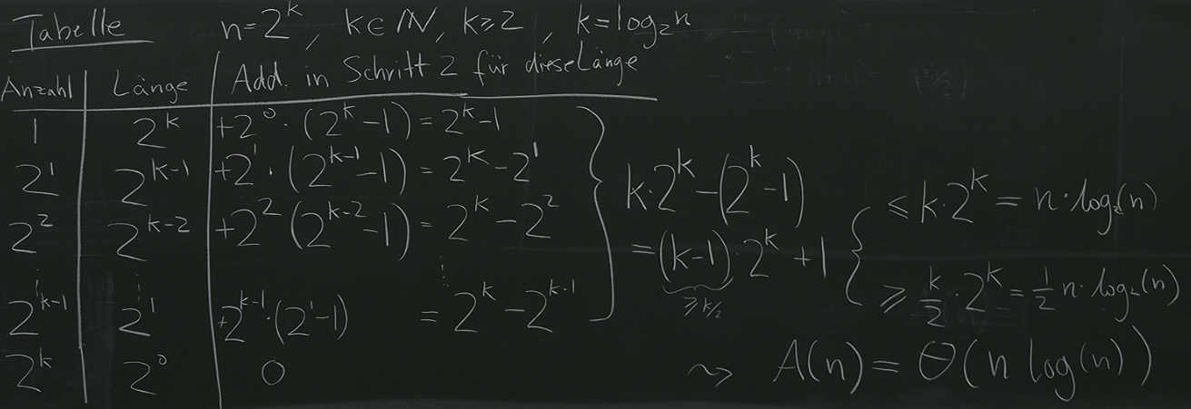
We can see that the time complexity $A(n)=\Theta (n\log (n))$. Buuut, geht es besser???

Algorithm 4: Differently recursively (Kadane’s algorithm)

Currently, we’ve been using the divide and conquer concept on the problem of $n\to \frac{n}{2}$. But what if we are able to instead do: $n\to n-1$?

Let us define $R_j:=ma{x}_{i\le j}{S}_{i,j}$, i.e. $R_j$ is the max sub array sum until there. Now we can observe that if we look at $R_{j-1}$ and want to find out $R_j$, we check if $R_{j-1}$ is positive, and if so, add it with the number at index $j$ to get $R_j$, if $R_{j-1}$ is negative, the number at index $j$ will be bigger, so we’ll start a “new subarray” starting there to calculate our further $R_j$‘s. This algorithm is called Kadane’s Algorithm.

Kadane’s Algorithm provides an efficient solution to the maximum subarray sum problem using dynamic programming. Instead of resorting to divide-and-conquer, Kadane’s Algorithm leverages dynamic programming to efficiently solve the maximum subarray sum problem. The core idea is to iteratively build up a solution by considering the contribution of each element to potential subarrays.

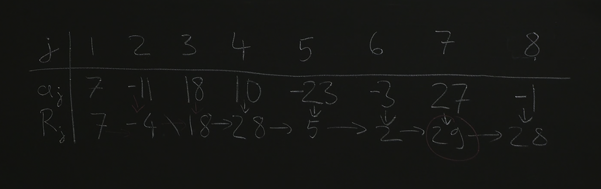
Let R[j] represent the maximum subarray sum ending at index j. We can express this recursively:

• Base Case: R[0] = a[0] (The maximum subarray sum ending at the first index is simply the value at that index).
• Recursive Step: R[j] = max(a[j], R[j-1] + a[j])
  • If starting a new subarray at index j yields a greater sum (a[j] ), then we update R[j].
  • Otherwise, we extend the previous subarray ending at index j - 1 by adding the current element (R[j-1] + a[j]), ensuring we consider both possibilities.

While recursion can be insightful, it often leads to redundant calculations. Kadane’s Algorithm is typically implemented iteratively for efficiency:

def max_subarray_sum(array):
    max_so_far = 0
    current_max = 0
    for i in range(len(array)):
        current_max = max(0, current_max + array[i])  # Extend or start a new subarray
        max_so_far = max(max_so_far, current_max) # Update overall maximum sum
    return max_so_far

Time complexity

This algorithm runs at $\Theta (n)$. This is because we iterate through the array only once to calculate the maximum subarray sum.

Buuut, geht es besser??? → Not really, because we can’t really skip look at each element and still calculate the max subarray sum. Every correct Algorithm for this problem must at least run $n$ reading operations and thereby must run at $\Theta (n)$.