01 Intro To Algorithms

Lecture from: 19.09.2024 | Video: Videos ETHZ | Rui Zhangs Notes

Algorithms are essential in computer science, especially when dealing with large data sets or solving complex problems. The goal of an algorithm is not just to solve a problem but to do so efficiently—minimizing the number of operations, execution time, and memory usage.

What is an Algorithm?

An algorithm is a step-by-step procedure for solving a problem. It breaks down a complex problem into smaller, simpler tasks that can be solved individually.

Computers can only perform basic operations—like addition or comparison—at incredible speed. When faced with a problem, we often consider multiple solutions and evaluate different algorithms based on their performance metrics: the number of operations, execution time, memory usage, etc.

Multiplication Algorithm

Let’s take an example we all know: the algorithm for multiplying two numbers using the traditional school method.

School Multiplication Algorithm

Example: Multiplying Two-Digit Numbers

Take two numbers, say 23 and 47. Here’s the basic process we learned in school:

1. Multiply the digits in the units place ($3\times 7=21$).
2. Multiply digits from the tens and units places, including zero padding ($2\times 7=14$ and $3\times 4=12$).
3. Multiply the digits in the tens place ($2\times 4=8$).
4. Sum up the results to get the final product.

This process essentially involves computing four partial products and then summing them up. Adding numbers is typically easier than multiplying them.

Example of 87 x 43:

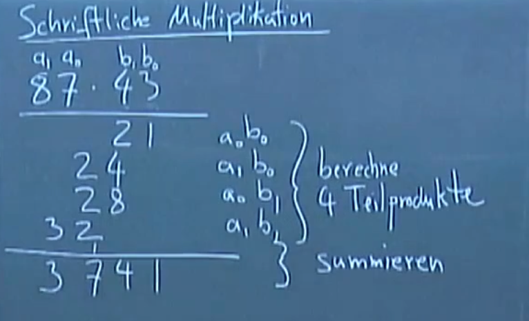
Correctness of the School Method

How do we know that this algorithm is correct? Let’s break down the math behind it. Consider the two-digit numbers:

$$(10a_1+a_0)(10b_1+b_0)$$

Expanding this using the distributive property:

$$(10a_1+a_0)(10b_1+b_0)=a_0{b}_0+10a_0{b}_1+10a_1{b}_0+100a_1{b}_1$$

This matches exactly with the operations we performed in the school method: the multiplication of the individual digits, followed by adding the correct powers of 10.

For n-digit numbers, the process is similar. We multiply each pair of digits and sum the results, adjusting for powers of 10 as needed.

Number of Operations in the School Method

If we multiply two n-digit numbers using this method, we perform $n\times n$ single-digit multiplications and a few additions. The total number of operations scales with $O(n^2)$—this means that multiplying two n-digit numbers takes approximately $n^2$ basic operations.

For example, multiplying two 1000-digit numbers would require about a million operations. While this approach is correct, it’s not the most efficient for large numbers.

Can We Do Better? (Geht es besser?)

Clearly, $O(n^2)$ becomes inefficient for large numbers, so mathematicians have explored algorithms that improve the speed of multiplication. One well-known improvement is Karatsuba’s algorithm, which reduces the complexity of multiplication to $O(n^{{\log }_{2}3})$, making it much faster for large numbers.

Karatsuba’s Algorithm

Karatsuba’s Algorithm is a more efficient method for multiplying large numbers than the traditional “school method.” It reduces the number of multiplications needed, improving the algorithm’s time complexity from $O(n^2)$ to $O(n^{{\log }_{2}3})\approx O(n^{1.585})$.

The key insight in Karatsuba’s Algorithm is to break down the multiplication of two n-digit numbers into smaller sub-problems. Instead of directly multiplying the numbers digit by digit, the algorithm divides each number into two parts, performs fewer multiplications, and then combines the results.

Recursive Algorithm Concept

At its core, Karatsuba’s Algorithm utilizes a recursive approach. Recursive algorithms solve a problem by breaking it down into smaller instances of the same problem. In this case, multiplying two n-digit numbers is transformed into multiplying two smaller numbers (each with approximately half the number of digits).

This concept can be summarized as follows:

1. Base Case: For small values of n (typically when n = 1), the algorithm performs direct multiplication, as it’s straightforward and efficient for single-digit numbers.

2. Recursive Step: For larger n, the algorithm splits each number into two halves. The multiplication is then expressed in terms of products of these halves, significantly reducing the number of multiplication operations required.

This recursive structure allows the algorithm to handle very large numbers efficiently. Each level of recursion handles a problem of smaller size until the base case is reached. As a result, this approach not only simplifies the calculations but also leverages the power of recursion to improve overall efficiency.

Algorithm Breakdown

Let’s multiply two n-digit numbers, $x$ and $y$. We can split $x$ and $y$ into two halves:

$$x=x_1\cdot 10^{n/2}+x_0$$ $$y=y_1\cdot 10^{n/2}+y_0$$

The product $x\cdot y$ can then be expressed as:

$$x\cdot y=(x_1\cdot 10^{n/2}+x_0)\cdot (y_1\cdot 10^{n/2}+y_0)$$

Expanding this gives:

$$x\cdot y=x_1{y}_1\cdot 10^n+(x_1{y}_0+x_0{y}_1)\cdot 10^{n/2}+x_0{y}_0$$

Karatsuba’s insight is to compute the middle term, $(x_1{y}_0+x_0{y}_1)$, more efficiently by using the following identity:

$$x_1{y}_0+x_0{y}_1=(x_1+x_0)(y_1+y_0)-x_1{y}_1-x_0{y}_0$$

Thus, instead of performing four multiplications ($x_1{y}_1$, $x_1{y}_0$, $x_0{y}_1$, and $x_0{y}_0$), Karatsuba’s method reduces this to just three multiplications:

1. $x_1{y}_1$
2. $x_0{y}_0$
3. $(x_1+x_0)(y_1+y_0)$

Then, the final result can be computed by combining these three products.

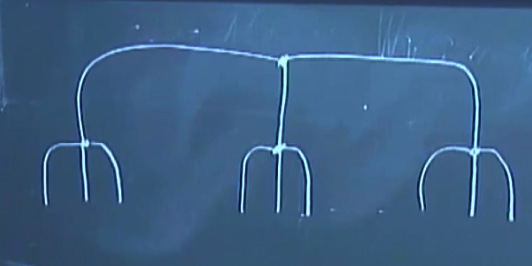
The recursiveness of this algorithm can be expressed as a tree:

Efficiency

In order to calculate the number of operations for n-digit numbers let us assume that the n-digit numbers have $2^k$ digits (and otherwise simply prepend 0s).

Using the recursive approach that divides multiplication into three smaller multiplications, we can analyze the number of single-digit multiplications required for multiplying two numbers of $n=2^k$ digits.

Using the recursive approach which divides a multiplication into three smaller multiplications. We break the multiplication of two $n$-digit numbers into three recursive multiplications of size $\frac{n}{2}$:

1. Compute $z_1=x_1{y}_1$
2. Compute $z_0=x_0{y}_0$
3. Compute $z_2=(x_1+x_0)(y_1+y_0)$

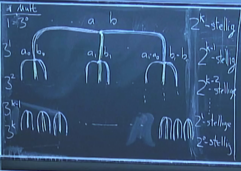
We can see that the multiplication of two $2^k$ digit number needs $3^k$ single-digit multiplications. Each of these multiplications is performed on numbers that have half the number of digits, leading to a recurrence relation for the time complexity:

$$T(n)=3T\left(\frac{n}{2}\right)+O(n)$$

Here, the $O(n)$ term accounts for the linear time needed to perform the additions and subtractions required to calculate $z_2$ and to combine the results.

To determine the time complexity from the recurrence, we can apply the Master Theorem. We compare $n^{{\log }_{b}a}$ with $O(n)$:

• $a=3$ (the number of subproblems),
• $b=2$ (the factor by which the size of the problem is reduced),
• $n^{{\log }_{b}a}=n^{{\log }_{2}3}$.

Calculating ${\log }_{2}3$ gives approximately $1.585$.

According to the Master Theorem, since $O(n)$ grows slower than $n^{{\log }_{2}3}$, we fall into the first case:

$$T(n)=\Theta (n^{{\log }_{2}3})$$

The school method needs $2^{2k}=4^k$. For $k=10$ the Karatsuba’s algorithm requires 10x less operations, for $k=20$ 100x less.

Karatsuba’s algorithm reduces the number of multiplications from $O(n^2)$ to $O(n^{{\log }_{2}3})$. This makes it significantly faster for large numbers than the “school” algorithm.

Summary of Efficiency

For two numbers with $n=2^k$ digits:

• Karatsuba’s Algorithm: Requires $3^k$ single-digit multiplications, leading to a complexity of $O(n^{{\log }_{2}3})$.
• School Method: Requires $4^k$ single-digit multiplications, leading to a complexity of $O(n^2)$.

Thus, when comparing the two algorithms:

• For $k=10$, Karatsuba’s algorithm requires approximately 10 times fewer operations than the school method.
• For $k=20$, it requires around 100 times fewer operations.

Overall, Karatsuba’s algorithm is significantly faster for large numbers, improving the multiplication efficiency by reducing the number of operations required.

Wall Following Algorithm (Pasture Break)

For this problem, our aim is to find a location along a 1D line by moving ourselves to it, with as few steps as possible.

Here a reason why you’d need this:

In a distant land, you find yourself trapped in an infinite, vast, circular arena, drawn here by an ancient prophecy. Legends say this place tests those who dare to enter, but you had no choice. Towering stone walls surround you, cold and endless. Though you’re not blindfolded, the arena is shrouded in darkness and thick fog, limiting your vision to just a few feet ahead. The air is damp, and every sound feels muted by the heavy mist.

The prophecy speaks of a single hidden passage along the arena’s perimeter, the only escape. You place your hands on the wall, feeling its rough, cold surface as you move carefully, searching for any change that might reveal the way out.

Wandering without a plan would be foolish. The prophecy offers a clue: The way is simple, though the path is unclear. Let your hands guide you.

(This is an Alternate Intro To “Pasture Break” or “the Wall Following Problem in 1D”)

In this problem our aim is to find the exit in as few steps as possible.

Algorithm 0 (Distance Given)

For this algorithm let us assume that someone has engraved into the wall infront of you that the exit is “k steps away”, however you don’t know which direction to go in. The most straightforward way to find the exit is to go k steps in the one direction, and if the exit isn’t there, then k steps back and k steps in the opposite direction.

• Best Case: k steps
• Worst Case: k steps + k steps back + k steps in the right direction = 3k steps

Algorithm 1 (Naive)

Now realistically, you won’t have any engraving telling you how far, nor in which direction that the exit is. You have to find this out on your own. The most simple algorithm would be:

• 1 left, back to start
• 2 right, back to start
• 3 left, back to start
• …
• k-1 right, back to start (we just missed the exit)
• k left, back to start
• k+1 right, but we stop after k, since we found the exit.

Now one of the ways to evaluate algorithms is to look at their worst case. So let us count how many steps we are doing.

$\text{Steps}=2\cdot 1+2\cdot 2+2\cdot 3+\cdots +2(k-1)+2k+k=k(k+1)+k$ We’ll compare this with the other algorithms later. Before that, let us try to think of a more clever algorithm.

Algorithm 2

The algorithm is:

• $2^0$ steps left, back to start
• $2^1$ steps right, back to start
• $2^3$ steps left, back to start
• …
• $2^{i-1}$ steps right, back to start
• $2^i$ steps left, back to start
• k (where $k>2^{i-1}$)

$$\text{Steps}=2\cdot 2^0+2\cdot 2^1+\cdots +2\cdot 2^{i-1}+2\cdot 2^i+k=2(2^{i+1}-1)+k$$

Comparison of Algorithms

In order to compare these algorithms we can’t have a mix of variables describing the steps required (worst case). In Algorithm 2 we currently have “k” and “i” as variables. Let us create an upper bounded inequality with only the variable k.

Upper Bound Algorithm 2

We can use the fact that:

$$k>2^{i-1}$$ $$2(2^{i+1})=8\cdot 2^{i-1}$$ $$8k>2(2^{i+1})⟹2(2^{i+1}-1)+k<8k-2+k<9k$$

Comparing

We can see that algorithm 1 has a worst case of $k(k+2)$ and algorithm 2 has a worst case of $9k$. Algorithm 2 thereby beats algorithm 1. There isn’t a algorithm which is faster (according to the prof).

Mathematical Induction

Mathematical induction is a powerful proof technique used to establish that a given statement is true for all natural numbers. The idea is similar to setting up a chain of falling dominoes: if you can show that the first domino falls (the base case) and that any domino will knock over the next one (the induction step), then you’ve proven that all dominoes will fall. Induction is a powerful tool in Algorithms and Data structures.

Steps of Induction

1. Base Step: Prove that the statement is true for the initial value (usually $n=1$).
2. Inductive Hypothesis: Assume that the statement is true for some arbitrary value $n=k$.
3. Inductive Step: Using the inductive hypothesis, prove that the statement is true for $n=k+1$.

Example: Sum of the First $n$ Natural Numbers

Let’s prove the formula for the sum of the first $n$ natural numbers:

$$1+2+3+\cdots +n=\frac{n(n+1)}{2}$$

Step 1: Base Case

For $n=1$, the left-hand side is simply $1$. Plugging $n=1$ into the formula:

$$\frac{1(1+1)}{2}=\frac{2}{2}=1$$

So, the base case holds.

Step 2: Inductive Hypothesis

Assume that the formula is true for some $n=k$:

$$1+2+3+\cdots +k=\frac{k(k+1)}{2}$$

Step 3: Inductive Step

Now we need to show that the formula holds for $n=k+1$. Consider:

$$1+2+3+\cdots +k+(k+1)$$

By the inductive hypothesis, the sum of the first $k$ terms is:

$$\frac{k(k+1)}{2}+(k+1)$$

Factor out $(k+1)$:

$$\frac{k(k+1)+2(k+1)}{2}=\frac{(k+1)(k+2)}{2}$$

This matches the formula for $n=k+1$:

$$\frac{(k+1)((k+1)+1)}{2}$$

Thus, by mathematical induction, the formula is true for all natural numbers $n$.

Example: Sum of Powers of 2

Let’s prove the formula for the sum of the first $n$ powers of 2:

$$2^0+2^1+2^2+\dots +2^n=2^{n+1}-1$$

Step 1: Base Case

For $n=0$, the left-hand side is:

$$2^0=1$$

Plugging $n=0$ into the formula:

$$2^{0+1}-1=2^1-1=2-1=1$$

So, the base case holds.

Step 2: Inductive Hypothesis

Assume that the formula is true for some $n=k$:

$$2^0+2^1+2^2+\dots +2^k=2^{k+1}-1$$

Step 3: Inductive Step

Now we need to show that the formula holds for $n=k+1$. Consider:

$$2^0+2^1+2^2+\dots +2^k+2^{k+1}$$

By the inductive hypothesis, the sum of the first $k$ terms is:

$$2^{k+1}-1+2^{k+1}$$

Combining these, we have:

$$(2^{k+1}-1)+2^{k+1}=2^{k+1}+2^{k+1}-1=2\cdot 2^{k+1}-1=2^{k+2}-1$$

This matches the formula for $n=k+1$:

$$2^{(k+1)+1}-1$$

Thus, by mathematical induction, the formula is true for all natural numbers $n$:

$$2^0+2^1+2^2+\dots +2^n=2^{n+1}-1$$