06 CR-Factorization and Linear Transformations

CR-Factorization

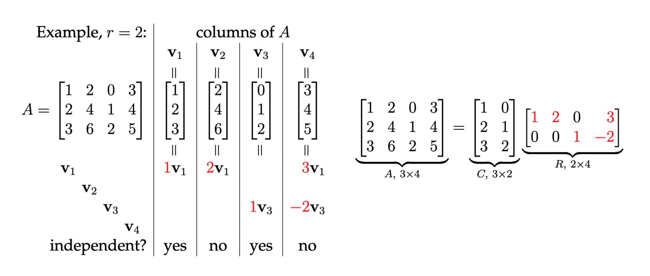
Imagine an $m\times n$ matrix, $A$, with a rank of r. This means its columns span an r-dimensional space. CR-Factorization says we can build $A$ from two special matrices:

• C: A smaller $m\times r$ matrix containing only the independent columns of $A$. These columns form a solid foundation, acting as a basis for the entire column space of $A$. Think of them as the “essential” building blocks.
• R: A unique $r\times n$ matrix that describes how the remaining columns of $A$ relate to these independent ones. It essentially encodes the “dependencies” between columns.

The beauty of CR-Factorization lies in this simple equation:

$$A=CR$$

This means we can reconstruct the original matrix, $A$, simply by multiplying $C$ and $R$.

In a Nutshell: CR-Factorization lets us represent a matrix as a combination of its fundamental building blocks ($C$) and the intricate web of relationships between its columns ($R$).

Example Rank 1 Matrix (Lemma 2.21)

Consider the matrix:

$$A=\left(\begin{array}{ccc}2& 4& 6\\ 3& 6& 9\end{array}\right)$$

This is a $2\times 3$ matrix where the rows are scalar multiples of each other, meaning the rank of the matrix is 1. We can express this matrix as the outer product of two vectors, which is a characteristic of rank 1 matrices.

According to Lemma 2.21, a matrix $A$ has rank 1 if and only if there exist non-zero vectors $v\in {\mathbb{R}}^m$ and $w\in {\mathbb{R}}^n$ such that:

$$A=v{w}^T$$

In this case, we can write:

$$v=\left(\begin{array}{c}2\\ 3\end{array}\right),w=\left(\begin{array}{c}1\\ 2\\ 3\end{array}\right)$$

The outer product $v{w}^T$ results in:

$$v{w}^T=\left(\begin{array}{c}2\\ 3\end{array}\right)\left(\begin{array}{ccc}1& 2& 3\end{array}\right)=\left(\begin{array}{ccc}2\cdot 1& 2\cdot 2& 2\cdot 3\\ 3\cdot 1& 3\cdot 2& 3\cdot 3\end{array}\right)=\left(\begin{array}{ccc}2& 4& 6\\ 3& 6& 9\end{array}\right)$$

Thus, we have successfully expressed matrix $A$ as the product of two vectors, confirming that it has rank 1.

Example Rank 2

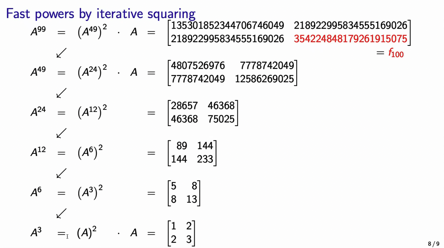
Fast Fibonacci Numbers by Iterative (Matrix) Squaring

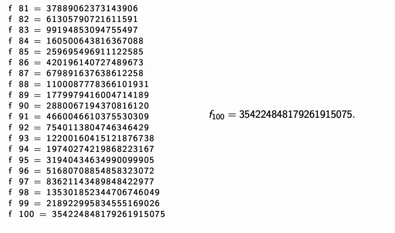
Now what if we wanted to find out $f_{100}$?

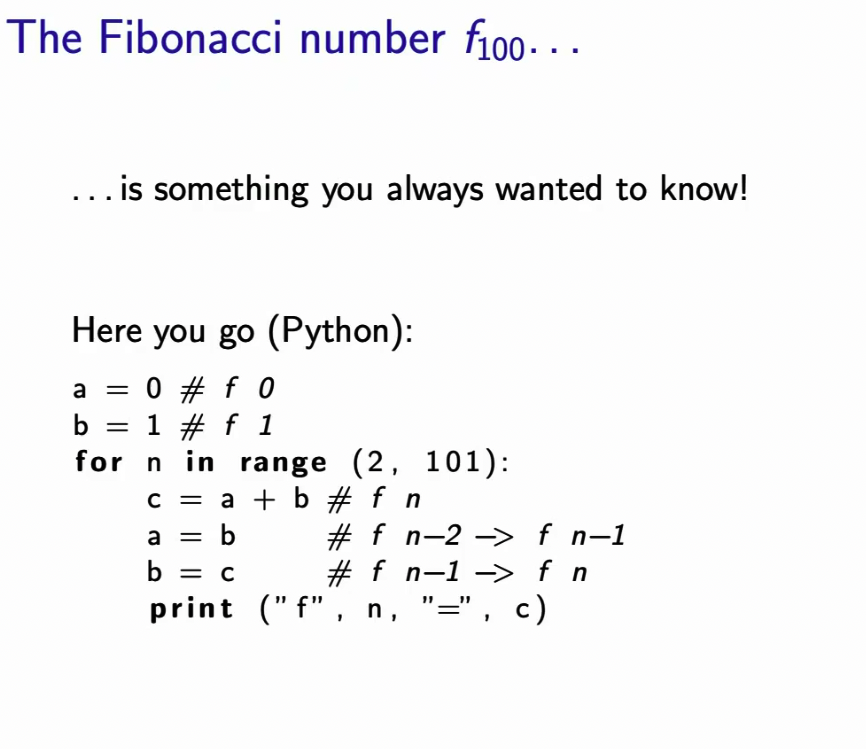
But this takes way to long. How can we do this faster?

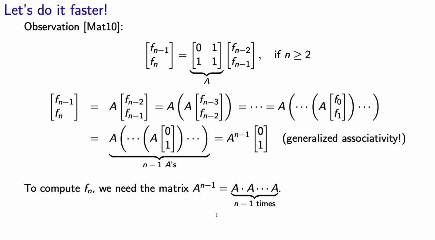
But now we’d have to compute $n-1$ matrix multiplications. We need to have a smarter way of doing that.

Matrices and Linear Transformations

A matrix can be thought of as a function or transformation that maps vectors from one vector space to another. This mapping adheres to the rules of linearity:

• Additivity: Transforming the sum of two vectors is equivalent to transforming each vector individually and then adding the results. Mathematically, for matrices A and vectors x, y:

  • $T_A(x+y)=T_A(x)+T_A(y)$

• Homogeneity: Scaling a vector by a scalar before transformation is equivalent to scaling the transformed vector. Mathematically, for a matrix A and vectors x, scalar λ:

  • $T_A(\lambda x)=\lambda T_A(x)$

These properties are crucial because they allow us to manipulate linear combinations of vectors efficiently using matrix operations.

The standard notation for this transformation is $Ax$, where A represents the matrix and x is the input vector. This product yields an output vector in a different vector space.

Input	Matrix	Output
$x\in {\mathbb{R}}^n$	$A\in {\mathbb{R}}^{m\times n}$	$Ax\in {\mathbb{R}}^m$

Here:

• $x\in {\mathbb{R}}^n$ : The input vector belongs to an n-dimensional Euclidean space.
• $A\in {\mathbb{R}}^{m\times n}$ : The matrix, A, is a rectangular array of real numbers with m rows and n columns. It defines the transformation between the spaces.
• $Ax\in {\mathbb{R}}^m$ : The output vector resides in an m-dimensional Euclidean space, reflecting the dimensionality change induced by the transformation.

Think of it this way: Matrices encapsulate linear transformations, enabling us to represent and manipulate complex geometric operations through efficient matrix calculations. This is fundamental in various fields like computer graphics, machine learning, and data analysis.

Example 1: Matrix Multiplication

If we have a matrix:

$$A=\left(\begin{array}{cc}1& 2\\ 3& 4\\ 5& 6\end{array}\right)$$

and an input vector:

$$x=\left(\begin{array}{c}1\\ 2\end{array}\right),$$

we can multiply them together. This multiplication is not like regular multiplication; it’s a specific process where we take each element of the matrix and combine it with corresponding elements from the vector. The result, $Ax$, is another vector:

$$Ax=\left(\begin{array}{c}1\cdot 1+2\cdot 2\\ 3\cdot 1+4\cdot 2\\ 5\cdot 1+6\cdot 2\end{array}\right)=\left(\begin{array}{c}5\\ 11\\ 17\end{array}\right).$$

Here, the matrix transformed the vector $x$ from ${\mathbb{R}}^2$ (two dimensions) to ${\mathbb{R}}^3$ (three dimensions).

Example 2: Linear Transformation

A linear transformation is a special type of function that preserves certain properties. We can represent it using a matrix. Let’s consider the transformation defined by this matrix:

$$A=\left(\begin{array}{cc}0& 1\\ 1& 0\end{array}\right).$$

This matrix “swaps” the components of a vector. Applying the transformation $T_A$ to a vector $x=\left(\begin{array}{c}{x}_1\\ x_2\end{array}\right)$ gives us:

$$T_A(x)=Ax=\left(\begin{array}{cc}0& 1\\ 1& 0\end{array}\right)\left(\begin{array}{c}{x}_1\\ x_2\end{array}\right)=\left(\begin{array}{c}{x}_2\\ x_1\end{array}\right).$$

So, if we input $\left(\begin{array}{c}3\\ 7\end{array}\right)$, the output is $\left(\begin{array}{c}7\\ 3\end{array}\right)$.

Visual Transformation

Let us define that a transformation of a set $X$ of inputs is defined as:

$T_A(X):=\{T_A(x):x\in X\}$

Example (${\mathbb{R}}^2\to {\mathbb{R}}^2$): “Space Distortion”:

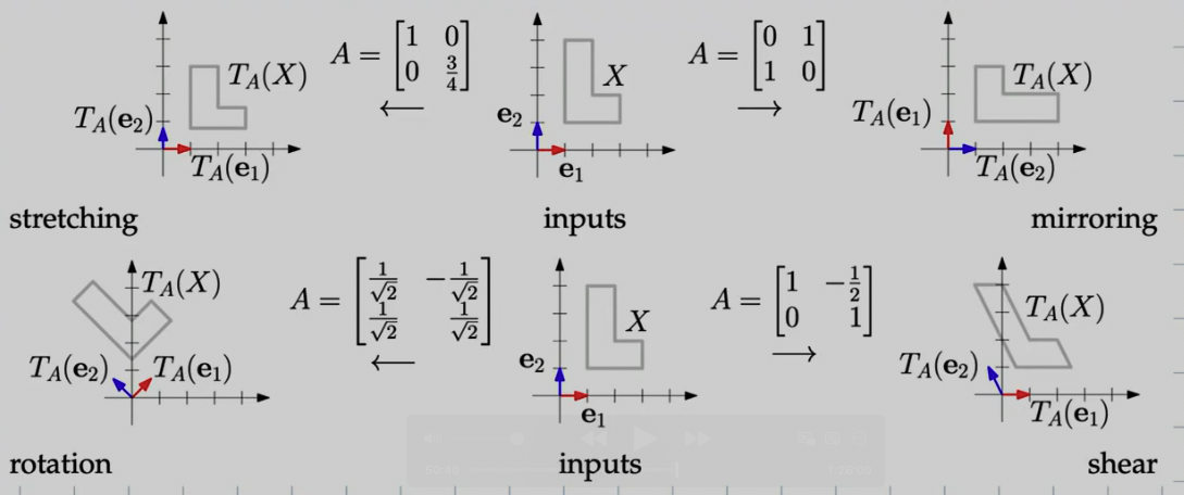
A simple way to think of what’s happening is to look at the unit vectors start and end position. 2D matrices allow you to operate on vectors in RR2 distort them by: stretching, mirroring, rotating, shearing,…

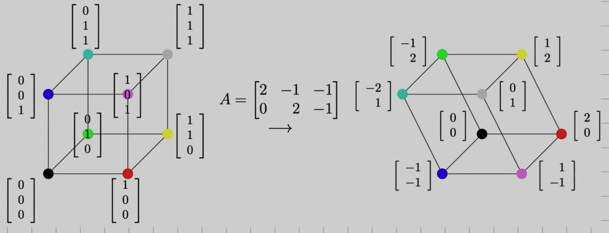
Example ${\mathbb{R}}^3\to {\mathbb{R}}^2$: “Orthogonal Projection”

Input 3D unit cube → Output: 2D Projection.

Linear Transformations Generalization

Linear transformations provide a powerful framework for describing how vectors can be transformed in a consistent and predictable manner.

A function $T:{\mathbb{R}}^n\to {\mathbb{R}}^m$ is considered a linear transformation if it satisfies the following two axioms for all vectors $\mathbf{x},\mathbf{y}\in {\mathbb{R}}^n$ and any scalar $\lambda \in \mathbb{R}$:

1. Additivity: $T(\mathbf{x}+\mathbf{y})=T(\mathbf{x})+T(\mathbf{y})$

2. Homogeneity: $T(\lambda \mathbf{x})=\lambda T(\mathbf{x})$

Examples

Linear Transformations Represented by Matrices:

1. Rotation in 2D: Rotating a vector in the plane by an angle θ can be achieved with the following 2x2 matrix:

$$\left[\begin{array}{cc}\cos (\theta )& -\sin (\theta )\\ \sin (\theta )& \cos (\theta )\end{array}\right]$$

2. Scaling in ℝ²: To scale a vector in the plane by a factor ‘k’ along both axes, we use the matrix:

$$\left[\begin{array}{cc}k& 0\\ 0& k\end{array}\right]$$

3. Projection onto the x-axis in ℝ²: This transformation maps any vector (x, y) to (x, 0). The corresponding matrix is:

$$\left[\begin{array}{cc}1& 0\\ 0& 0\end{array}\right]$$

4. Shearing in ℝ²: Shearing a vector distorts its shape by moving points along diagonal lines. A common shear transformation can be represented with the matrix:

$$\left[\begin{array}{cc}1& s\\ 0& 1\end{array}\right]$$

where ‘s’ is the shearing factor.

Linear Transformations Without Matrices:

1. Differentiation: The derivative of a function (e.g., $f^{\prime }(x)$) is a linear transformation because:

   • It satisfies additivity: $D(f(x)+g(x))=f^{\prime }(x)+g^{\prime }(x)$
   • It satisfies homogeneity: $D(cf(x))=c\ast f^{\prime }(x)$

2. Integration: Similar to differentiation, the integral of a function (e.g., $\int f(x)dx$) is also a linear transformation.