01 Vectors

Lecture from: 18.09.2024 | Video: Videos ETHZ

Basic Operations

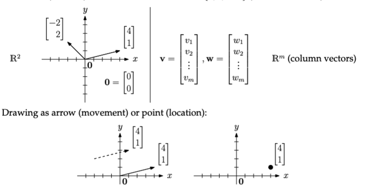
What is a vector

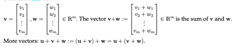
A vector is a element in ${\mathbb{R}}^n$. Vectors can be visualised as arrows going from the origin to their coordinate.

Addition

Vector addition only works when both vectors have the same dimension (you can’t add a 3-dimensional vector to a 10-dimensional one).

To add vectors, simply add their corresponding elements, resulting in a new vector of the same dimension.

Vector addition is commutative, meaning the order in which you add them doesn’t matter. You can visualize it by placing one vector at the end of the other (where the arrow points) and following that path.

Scaling

Vectors can be scaled by multiplying each of their individual elements by a scalar factor. Scaling is a commutative property, meaning the order of operations doesn’t affect the result.

If you scale a vector $\mathbf{v}=[v_1,v_2,v_3]$ by a factor of $k$, the resulting vector is $\mathbf{kv}=[k\cdot v_1,k\cdot v_2,k\cdot v_3]$.

Linear Combinations

A linear combination of a set of vectors involves creating a new vector by multiplying each vector by a scalar (coefficient) and then summing the results.

Given vectors ${\mathbf{v}}_1,{\mathbf{v}}_2,\dots ,{\mathbf{v}}_{\mathbf{n}}$ and corresponding scalars $c_1,c_2,\dots ,c_n$, the linear combination is expressed as:

$$\mathbf{L}=c_1{\mathbf{v}}_1+c_2{\mathbf{v}}_2+\dots +c_n{\mathbf{v}}_{\mathbf{n}}$$

The resulting vector $\mathbf{L}$ can represent any point in the span of the original vectors, depending on the choice of the coefficients.

Visual Representations

Suppose you have a resulting vector from a linear combination of vectors, and you want to find its coefficients. There are two ways to think of these coefficients visually: through the row picture and the column picture.

Row Picture

In the row picture, you can visualize each vector as a row in a matrix. The unknown coefficients are represented as a vector, and the resulting vector is obtained by multiplying the coefficient vector by the matrix of vectors. This leads to a system of linear equations, where each equation corresponds to a row in the matrix. The equations can be expressed as:

$$\begin{array}{rl}{c}_1\cdot v_{11}+c_2\cdot v_{12}+\dots +c_n\cdot v_{1n}& =L_1\\ c_1\cdot v_{21}+c_2\cdot v_{22}+\dots +c_n\cdot v_{2n}& =L_2\\ & ⋮\\ c_1\cdot v_{m1}+c_2\cdot v_{m2}+\dots +c_n\cdot v_{mn}& =L_m\end{array}$$

Here, ($L$) represents the components of the resulting vector, and ($v_{ij}$) represents the components of the original vectors. Now each of these rows can represented by a line in a coordinate system. If all of your lines intersect at a point, you’ve found your coefficients.

Column Picture

In the column picture, you visualize the vectors as columns of a matrix. The resulting vector is expressed as a linear combination of these column vectors, with the coefficients determining how much of each column vector contributes to the final vector. This can be represented as:

$$\mathbf{L}=c_1\left(\begin{array}{c}{v}_{11}\\ v_{21}\\ ⋮\\ v_{m1}\end{array}\right)+c_2\left(\begin{array}{c}{v}_{12}\\ v_{22}\\ ⋮\\ v_{m2}\end{array}\right)+\dots +c_n\left(\begin{array}{c}{v}_{1n}\\ v_{2n}\\ ⋮\\ v_{mn}\end{array}\right)$$

The resulting vector $\mathbf{L}$ is a linear combination of the column vectors, and the coefficients tell you how much to “weigh” each column vector in producing the resulting vector. Visually these can be thought of a combination of “arrows” added finally resulting in our resulting vector $\mathbf{L}$

Both representations provide valuable insights into the relationships between the vectors and their coefficients, and they are useful tools for solving linear systems.

Special Linear Combinations

Linear combinations can be specialized depending on the restrictions placed on the coefficients. These special types — affine, conic, and convex combinations — give rise to important geometric and algebraic interpretations.

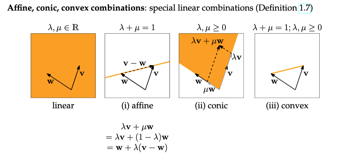
Affine Combination

An affine combination of vectors allows for linear combinations, but with the added restriction that the sum of the coefficients must equal 1. This keeps the result “anchored” within the same geometric space, ensuring that you don’t drift too far from the set of original vectors.

Given vectors ${\mathbf{v}}_1,{\mathbf{v}}_2,\dots ,{\mathbf{v}}_{\mathbf{n}}$, an affine combination looks like:

$$\mathbf{L}=c_1{\mathbf{v}}_1+c_2{\mathbf{v}}_2+\dots +c_n{\mathbf{v}}_{\mathbf{n}}$$

with the condition that:

$$c_1+c_2+\dots +c_n=1$$

Intuitive Understanding: Imagine the vectors are points on a flat plane. The affine combination allows you to “move” between these points in a way that stays confined to the plane spanned by the vectors. For example, in 2D, if you take an affine combination of two points (vectors), you’ll be somewhere on the line connecting those two points.

Conic Combination

In a conic combination, the coefficients must be non-negative, meaning $c_i\ge 0$, but there’s no requirement that their sum equals 1. This allows for combinations that scale outward, similar to a “cone” extending from the origin.

A conic combination is expressed as:

$$\mathbf{L}=c_1{\mathbf{v}}_1+c_2{\mathbf{v}}_2+\dots +c_n{\mathbf{v}}_{\mathbf{n}}$$

with the condition that:

$$c_i\ge 0\text{for all}i$$

Intuitive Understanding: Think of the original vectors as defining directions, and a conic combination allows you to travel any distance along those directions. Because the coefficients are non-negative, you can only move forward, never backward. The result is that you “fan out” along the directions of the vectors, like rays from the origin.

Convex Combination

A convex combination combines the restrictions of both affine and conic combinations. The coefficients must sum to 1 (like affine combinations), and they must also be non-negative (like conic combinations). This confines the result to the interior of the shape spanned by the vectors.

A convex combination looks like:

$$\mathbf{L}=c_1{\mathbf{v}}_1+c_2{\mathbf{v}}_2+\dots +c_n{\mathbf{v}}_{\mathbf{n}}$$

with the conditions that:

$$c_1+c_2+\dots +c_n=1\text{and}{c}_i\ge 0\text{for all}i$$

Intuitive Understanding: Picture the vectors as points, and a convex combination is like finding a point inside the “shape” formed by these vectors. If you have two vectors, their convex combination places you somewhere along the line segment connecting them. With three vectors, the convex combination keeps you inside the triangle formed by those vectors. For four vectors, you’re inside the tetrahedron, and so on. You can’t “escape” the region bounded by the vectors because of the non-negative coefficients and the sum-to-1 condition.

Continue here: 02 Vectors