05 Sorting, Data Structures

Lecture from: 17.10.2024 | Video: Videos ETHZ | Rui Zhangs Notes | Official Script

Sorting Algorithms

In the past lecture we looked at various different sorting algorithms. We forgot to ask our favourite question: Geht es besser?

And the answer actually is no (for comparison based algorithms). The best we can have is $O(n\log (n))$.

If we similar to our previous lecture imagine a decision tree showing us comparison then the depth of tree is showing us the amount of comparisons we’d need to do in a worst case. The maximal number of nodes at the very bottom is maximally $2^{h+1}$.

Notice, it must be given that the number of nodes must be as big or bigger than the number of possible permutations of our input array. The number of permutations for an array of size $n$ is $n!$. So currently we have:

$$2^{h+1}\ge \text{number of nodes}\ge \text{possible permutations}=n!$$ $$⟹h={\log }_2(n!)-1\in \Omega (n\log (n))$$

We have hereby shown that merge sort for instance is an optimal algorithm. Now, even if we have a “optimal” algorithm, we’ll still look at other different algorithms, in order to have more options and ideas about these algorithmic patterns which we can then use in future similar problems.

Quicksort

Quicksort is another efficient sorting algorithm that, like Merge Sort, uses the divide and conquer strategy. However, unlike Merge Sort, it sorts the elements in place (i.e., it doesn’t require additional space for merging). Quicksort is known for its average case performance of $O(n\log n)$ and its simplicity in implementation.

How Quicksort Works:

1. Divide (Partition Step):

   • The algorithm chooses an element from the array, called the pivot.
   • It then reorders the array such that all elements smaller than the pivot are moved to the left of the pivot, and all elements greater than the pivot are moved to the right. This process is called partitioning.
   • After partitioning, the pivot is in its correct position in the sorted array.

2. Conquer:

   • Recursively apply the same process (choosing a pivot and partitioning) to the left and right subarrays (those smaller and greater than the pivot).

3. Combine:

   • Since the subarrays are already sorted, no combining step is needed. The sorted array is produced once all recursive calls are complete.

Pseudocode:

function quicksort(A, low, high):
    if low < high:
        pivot = partition(A, low, high)  # Partition the array and get the pivot's index
        quicksort(A, low, pivot - 1)     # Recursively sort the left subarray
        quicksort(A, pivot + 1, high)    # Recursively sort the right subarray
 
function partition(A, low, high):
    pivot = A[high]                    # Choose the last element as the pivot
    i = low - 1                        # Index of smaller element
    for j in range(low, high):
        if A[j] <= pivot:
            i += 1                     # Increment the index of the smaller element
            A[i], A[j] = A[j], A[i]     # Swap
    A[i + 1], A[high] = A[high], A[i + 1]  # Place pivot in the correct position
    return i + 1                       # Return the pivot's final position

Runtime

We’ll notice that the recursion step depends on where the pivot element lands. We might have a good runtime, but we might also have picked the pivot to actually be the element at the very right/left, giving us different runtimes.

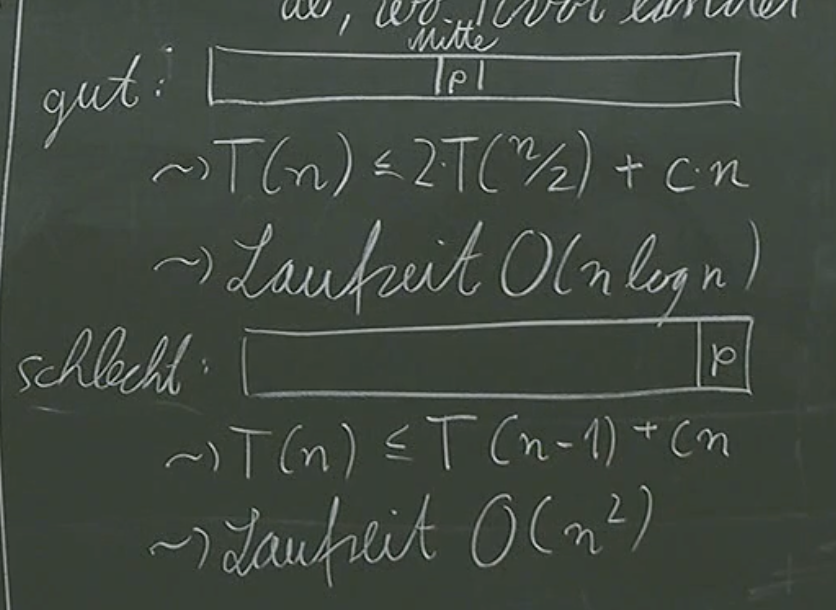
You can see the worst case is $O(n^2)$. There is a solution to this problem, but we’ll only learn about it in next semester. The idea however is that we randomly choose a pivot element and by doing that we’ll be in the “good” case.

You’ll see that it becomes virtually impossible for us to get $O(n^2)$ and that the average case will be $O(n\log n)$.

Heap Sort

Let’s first look at selection sort from last lecture. You might recall that our invariant was that the last $n$ elements of our array are sorted correctly, and then we select the next max element from the remaining array and put it in it’s place. This task of finding the max element in an array was running at $O(n)$ which finally contributed to our algorithms runtime of $O(n^2)$.

Our new idea for heap sort is to arrange our data in such a way, where we find the max element quickly. The data structure used to store our data in such a way is called a heap.

Our max-heap is going to arrange our data in a tree-like structure.

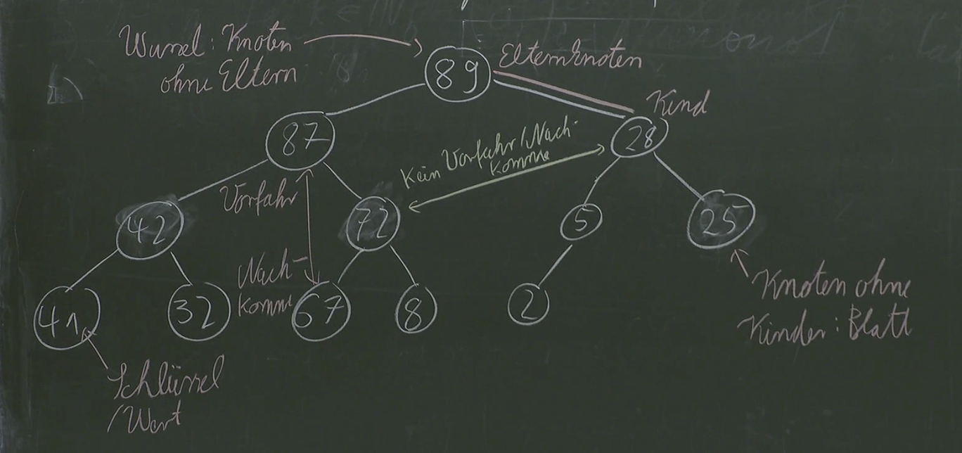
Our tree-like structure cannot be an arbitrary tree, but needs to be an exact: complete binary tree. Let’s explain:

• binary: each node can have 2 child nodes
• complete: all nodes except leaf nodes must have 2 child nodes and the last “level” is filled up left to right.

Heap Condition: The value of a node must be larger than the value of it’s children:

• $value(node)\ge value(children)$
• $value(ancestor)\ge value(descendents)$ by transitivity

Given such a tree, we know that the max is always at the root of the tree.

Now this is a nice idea with which we might be able to improve “selection sort”. But we need to specify:

1. How to Array -> Heap (Complete Binary Tree)
2. Find the max and remove it from the heap.

So currently our algorithm might look something like this:

function HeapSort(A):
	H = createHeap(A #todo
	for i in range(n,1,-1):
		A[i] = extractMax(H) #todo

Now let’s tackle the first problem: extracting the maximum.

Extract Max

In order to get the maximum, we can simply take and delete the root element of our tree. But then we got a problem, we have 2 trees. In order to solve that, let us go and pick the last element in the last element (i.e. if you imagine the tree as a triangle, take the element at the most bottom right part) and then put it in the place where you “deleted” the root node.

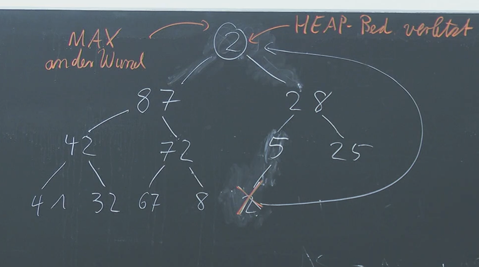
Now we do technically have a binary tree, but the heap condition (children value must be smaller or equal to nodes value) is not not fulfilled. To “fix” this, let us simply switch the positions of our current wrong root node with the max of it’s children.

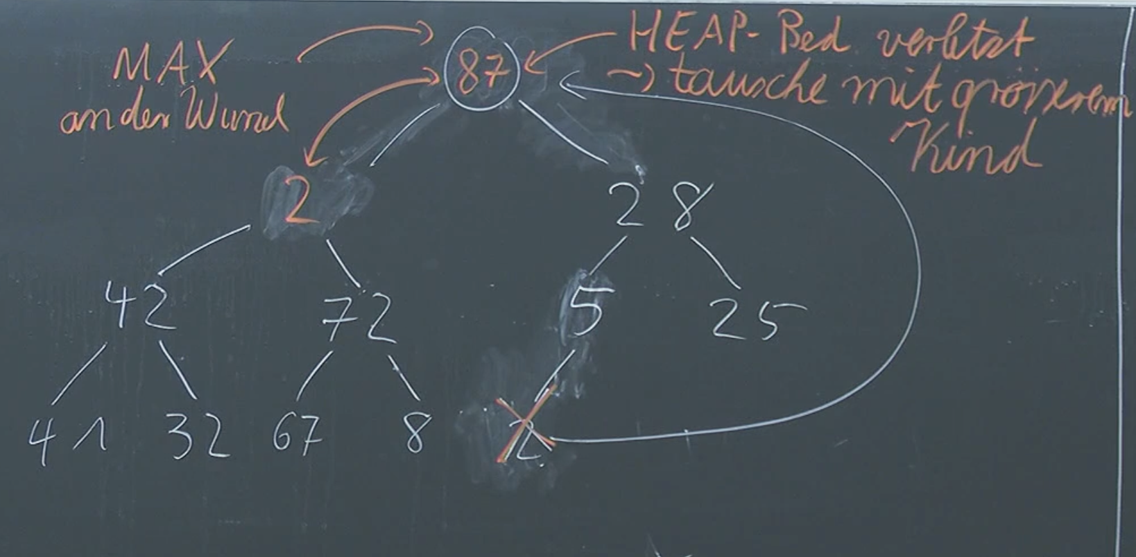
Now we simply moved our problem down a level. Our heap condition is satisfied everywhere except in one of the nodes. Trivially, we simply iteratively repeat the switching of nodes until we don’t have a problem, i.e the heap condition is satisfied everywhere. So in essence:

function extractMax(H):
	max = popRoot(H)
	lastElement = popBottomRight(H)
	setRoot(lastElement)
	isSatisfied = False # in the beginning it most definitely will not be satisfied
 
	while !isSatisfied:
		largestChild = getMax(lastElement.children)
		if largestChild.value > lastElement.value:
			H.switch(largestChild, lastElement)
			
		isSatisfied = lastElement.children.forall((child)=>{
			child.value <= lastElement.value
		})

The runtime of our algorithm is $O(h)$ where $h$ is the height of our tree, which then resolves to $O(\log n)$.

Create Heap

Let us start with an empty heap, and then we’ll add nodes one after the other. Let us look at how to insert a new node.

To insert, the most simply way to preserve the tree structure is to simply add our node to the bottom right empty position.

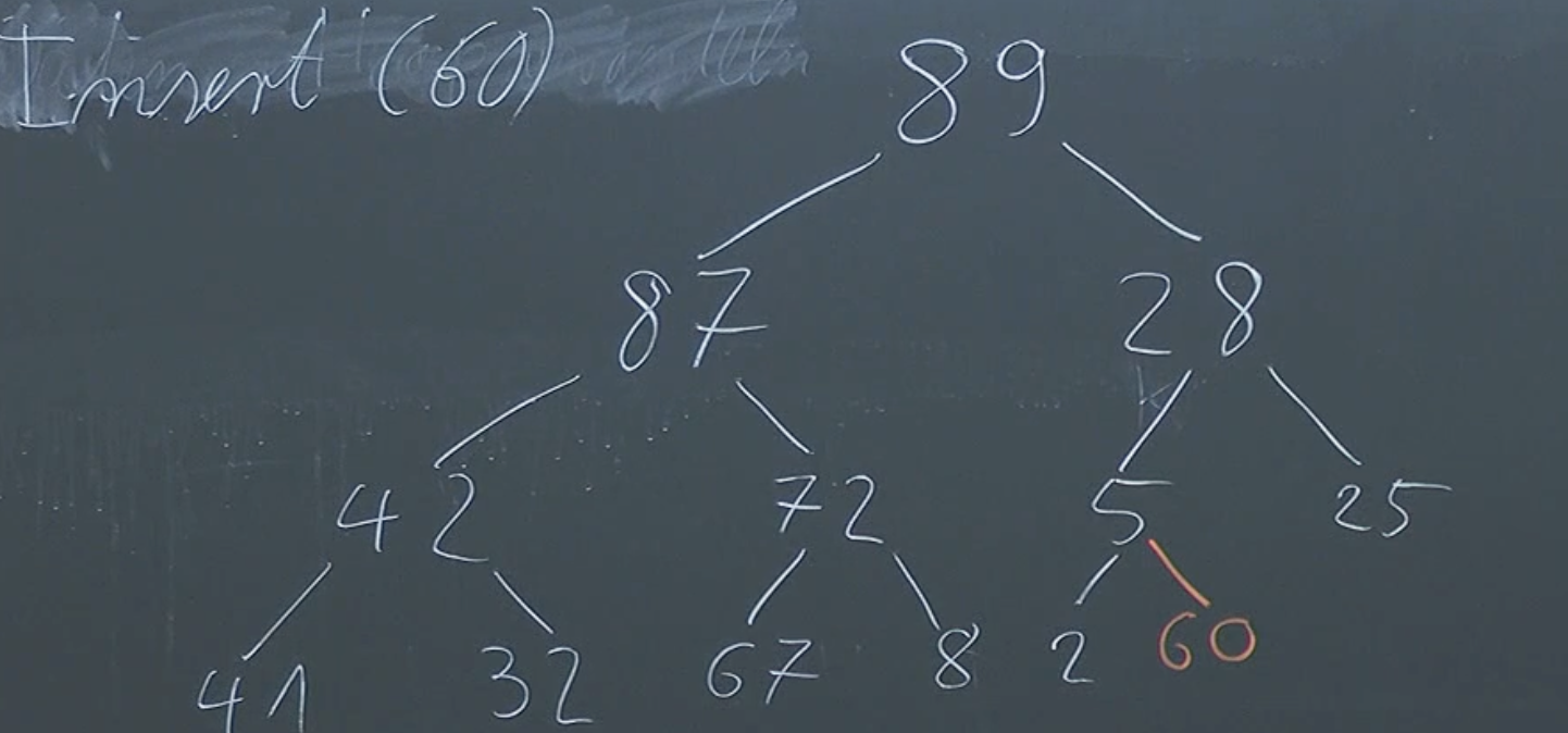
But now we’ve not satisfied our heap condition. Similar to extracting the max, we’ll simply “fix” our problem by switching with parent nodes, until our heap condition is satisfied everywhere.

function insert(H, node):
	element = pushEmptyBottomRight(H, node)
	while element.parent && (element.value > element.parent.value):
		H.switch(element, element.parent)

Our insertion function runs at $O(\log n)$ Now by defining our insert function, we can easily create a heap.

function createHeap(A):
	H = new Heap()
	A.foreach((v)=>{
		insert(H, v))
	})

Creating runs at $O(n\log n)$.

Storing Our Heap

A very important question we need to think of is how we actually want to store our heap. One simple way of doing this is to use an array and have the first element be the root, the next two it’s children, the next 4 the next children… Effectively we are concatenating the heaps levels in a single array.

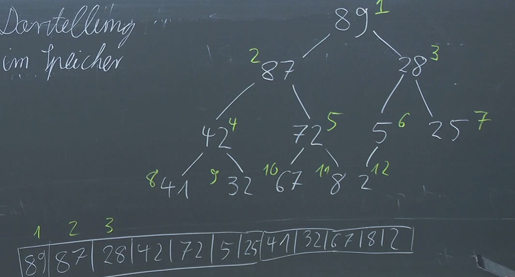
We can see that the children of $A[k]$ are at $A[2k]$ and $A[2k+1]$.

Runtime

Quite simple, we are inserting $n$ times and extracting $n$ times. Insertion and extraction run at $O(\log n)$. Together the whole thing runs at $O(n\log n)$, as fast as merge sort and quick sort.

Data Structures

A data structure is a specialized way of organizing and storing data in a computer so that it can be accessed and modified efficiently.

We differentiate between Abstract Data Types and Data Structures:

An abstract data type (ADT) deals with:

• What is this data structure
• What operations can I do (e.g. insert, extract, find,…)

A data structure deals with:

• How do we actually want to store the ADT in memory/… on our computer.

Example: Abstract Data Type - List

Lists are a collection of elements, each identified by an index or key.

Operations:

• append(val) to list
• get(ith) from list
• insert(val, index) into list
• …

Data Structures for ADT List:

1. Array (fast retrieval, slow insertion)
2. Linked List (fast insertion/deletion, slow retrieval)

Continue here: 06 Abstract Data Types, Binary AVL Search Trees