06 Abstract Data Types, Binary AVL Search Trees

Lecture from: 22.10.2024 | Video: Videos ETHZ | Rui Zhangs Notes | Official Script

Abstract Data Types

Last time, we discussed abstract data types and how various data structures can implement them. We saw that lists aren’t ideal for dictionaries due to their inefficient insertion and search operations. Today, we’ll explore binary trees as a more suitable solution.

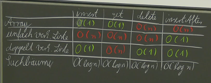
ADT: Dictionary

A dictionary is a collection of unique keys with the following operations:

• search(x, D): Returns true if integer x exists in dictionary D, otherwise false.
• insert(x, D): Adds key x to D only if it doesn’t already exist.
• delete(x, D): Removes key x from D.

Binary Trees (for Dictionaries)

We can implement dictionaries using binary trees. A binary tree satisfies these conditions:

• All keys in the left subtree are smaller than the root node’s key.
• All keys in the right subtree are larger than the root node’s key.

This structure enables efficient searching, insertion, and deletion.

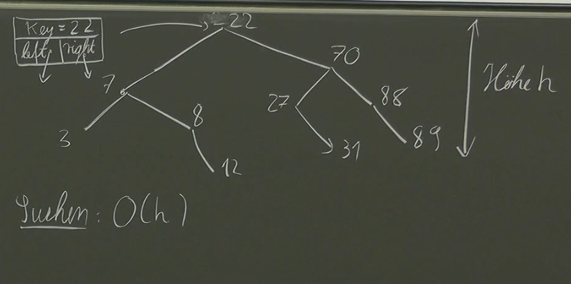
Searching ($O(\log n)$)

To search for a key x in a binary tree:

1. Start at the root node.
2. Compare x with the root’s key.
3. If x is equal to the root’s key, we found it! Return true.
4. If x is smaller than the root’s key, recursively search the left subtree.
5. If x is larger than the root’s key, recursively search the right subtree.
6. If we reach a leaf node and haven’t found x, return false.

Insertion ($O(\log n)$)

1. Start at the root node.
2. Traverse the tree, comparing x with each node’s key.
3. If x is equal to an existing key, we already have it! Return false (prevent duplicates).
4. If we reach a leaf node:

• Insert x as a new node in the appropriate position (left or right) based on its value compared to the parent node’s key.

Deletion ($O(\log n)$)

Deleting a node in a binary tree is more complex and requires careful handling of potential issues like orphaned nodes and maintaining the binary search tree property.

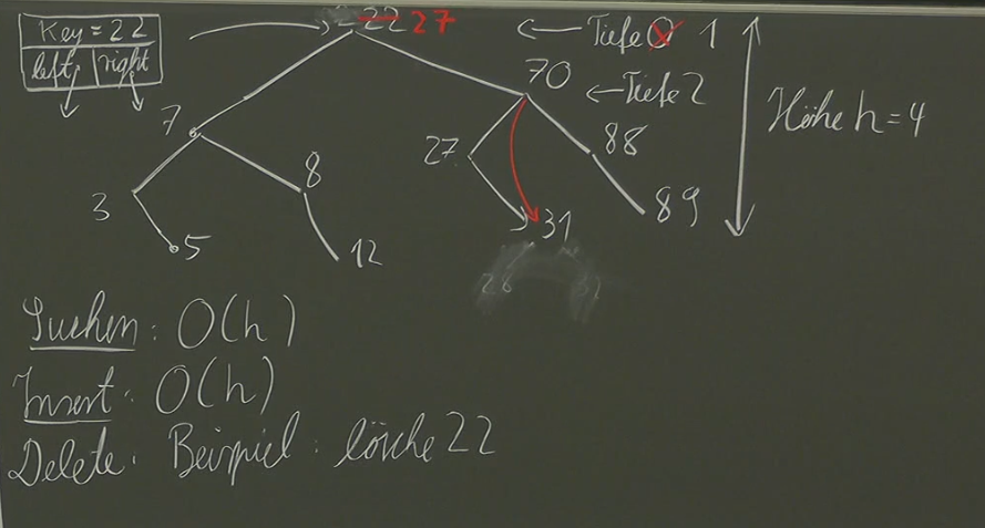
1. Find the Node: Locate the node to be deleted using search algorithm.
2. Case 1: Node with No Children or One Child:
   • Simply remove the node and connect its parent directly to its child (if any).
3. Case 2: Node with Two Children:
   • Find the inorder successor (smallest key in the right subtree) of the node to be deleted.
   • Replace the node’s value with its inorder successor’s value.
   • Delete the inorder successor from its original position.

Problem: The Linearised Binary Search Tree

The current binary search tree implementation has a critical flaw when dealing with sequential insertion. If we insert values in ascending order, the resulting structure becomes more like a linked list than a balanced tree.

Consider inserting the following sequence of values into an empty binary search tree: 2, 3, 4, .... Due to the inherent nature of binary search trees, each new node will be placed as the right child of the previous node. This leads to a linear structure where nodes are connected only through their right children, effectively creating a degenerate case of a binary search tree.

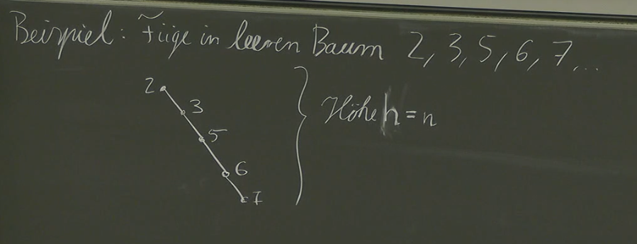
This linearization significantly degrades the performance benefits of a binary search tree, as searching, insertion, and deletion operations all revert to O(n) complexity – similar to a simple linked list.

Complete Binary Search Trees (Idea 1)

One might initially consider enforcing completeness, similar to a max heap, where each level of the tree is completely filled except possibly the last level which is filled from left to right. This approach suggests maintaining a complete binary search tree and inserting new elements in a way that preserves this property.

However, this idea presents several challenges:

• Limited Flexibility: A complete binary search tree imposes strict structural constraints. With n elements, there’s only one valid configuration for the tree. This rigidity makes insertions complex, as they might necessitate shifting numerous nodes to maintain completeness.
• Inefficiency: The effort required to shift nodes during insertion could outweigh the benefits of a complete structure.

Ultimately, this approach proves inefficient and inflexible for dynamic data structures like dictionaries.

Binary AVL Search Trees (Idea 2)

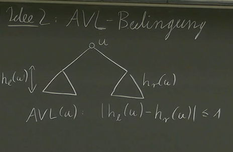
The AVL condition offers a more promising solution to maintain balance in our binary search tree.

An AVL tree is defined by the following property: For every node in the tree, the height difference between its left and right subtrees is at most 1 ($|h_l-h_r|\le 1$). This self-adjusting nature ensures that the tree remains relatively balanced, even after repeated insertions and deletions.

Indeed, visually inspecting different trees to determine if they are AVL trees can be challenging:

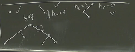
To streamline this process, we’ll introduce h_l and h_r attributes to our nodes, storing the heights of the left and right subtrees respectively:

This modification provides us with two key questions to address:

1. Tree Height: How do we determine the height of an AVL tree? We know it is O(log n).
2. Restoration After Operations: How do we modify the tree after insertion or deletion operations to ensure the AVL condition remains satisfied?

Let’s consider question 1: Given a height h of an AVL tree, how many nodes can it hold? A fascinating result emerges: an AVL Tree of height h has at least Fib(h+2) - 1 nodes.

Proof by Induction:

• Base Case (h = 0): An AVL tree of height 0 has a single node, satisfying the condition Fib(0+2) - 1 = 1.
• Inductive Hypothesis: Assume an AVL tree of height k has at least Fib(k+2) - 1 nodes.
• Inductive Step: Consider an AVL tree of height k+1. To maintain the AVL condition, its left and right subtrees must have heights between k and k-1. By the inductive hypothesis, each subtree has at least Fib(k+1) - 1 nodes. Therefore, the entire tree has at least 2 * (Fib(k+1) - 1) + 1 nodes = Fib(k+3) - 1 nodes.

This proof highlights the inherent efficiency and structural properties of AVL trees.

We can further analyze this relationship: We see that $n\ge Fib(h+2)\ge \frac{1}{3}1.5^{h+2}$ → $h\le {\log }_{1.5}(3(n+1))-2⟹\in O(\log n)$. This implies that the height of an AVL tree is logarithmic in terms of the number of nodes it contains.

Insertion and Repairing

While inserting a new node into an AVL tree might not always violate the AVL condition, there are scenarios where it does. Remember, only the predecessors and ancestors of the inserted node can potentially disrupt the balance; unrelated nodes remain unaffected.

Our strategy for handling these disruptions involves a systematic check: we traverse the tree from bottom to top, examining each node’s height difference between its left and right subtrees. If the AVL condition ($|h_l-h_r|\le 1$) is violated, we initiate a repair process.

This repair process hinges on identifying the specific type of imbalance:

• LL Case: The inserted node’s grandparent has a right subtree that’s taller than its left subtree by at least two levels.
• LR Case: The inserted node’s grandparent has a left subtree that’s taller than its right subtree by at least two levels, and the inserted node is on the right side of its parent.
• RR Case: Similar to LL, but with the roles of left and right subtrees reversed.
• RL Case: Similar to LR, but with the roles of left and right subtrees reversed.

Each case necessitates a distinct rotation sequence to restore the AVL property.
Here are the corrected descriptions for all four AVL tree repair cases:

Repair Cases and Rotations in AVL Trees

In AVL trees, when an insertion causes an imbalance, it affects three key nodes: A, the nearest unbalanced ancestor; B, the child of A; and C, the grandchild of A where the new node was inserted. Each imbalance type has a specific rotation pattern to restore balance. Below are the four possible cases:

LL Case (Left-Left Imbalance)

In the LL case, the imbalance occurs because the left subtree of A’s left child B is too tall. To restore balance, we perform a right rotation on A.

• Steps for Right Rotation:
  1. Identify nodes A, B, and C, where A is the unbalanced node, B is A’s left child, and C is B’s left child.
  2. Perform a right rotation on A, making B the new root of this subtree.
  3. B’s right child (if any) becomes the left child of A.
  4. Set A as the right child of B.

This rotation decreases the left subtree height of A, restoring the AVL property.

LR Case (Left-Right Imbalance)

In the LR case, A’s left subtree is too tall, but the newly inserted node is in the right subtree of A’s left child, B. To fix this, we perform a left rotation on B followed by a right rotation on A.

• Steps for Left-Right Rotation:
  1. Identify nodes A, B, and C, where A is the unbalanced node, B is A’s left child, and C is B’s right child.
  2. Perform a left rotation on B, making C the left child of A.
  3. Then perform a right rotation on A, making C the new root of this subtree.

This double rotation balances the subtree by shifting nodes to appropriate positions.

RR Case (Right-Right Imbalance)

In the RR case, the imbalance is due to A’s right subtree being too tall, specifically in the right subtree of B. We correct this with a left rotation on A.

• Steps for Left Rotation:
  1. Identify nodes A, B, and C, where A is the unbalanced node, B is A’s right child, and C is B’s right child.
  2. Perform a left rotation on A, making B the new root of the subtree.
  3. B’s left child (if any) becomes the right child of A.
  4. Set A as the left child of B.

The left rotation reduces the height of A’s right subtree, restoring AVL balance.

RL Case (Right-Left Imbalance)

In the RL case, A’s right subtree is too tall, with the newly inserted node positioned in A’s right child B’s left subtree. To balance this, we perform a right rotation on B followed by a left rotation on A.

• Steps for Right-Left Rotation:
  1. Identify nodes A, B, and C, where A is the unbalanced node, B is A’s right child, and C is B’s left child.
  2. Perform a right rotation on B, making C the right child of A.
  3. Then perform a left rotation on A, making C the new root of this subtree.

This double rotation realigns nodes to maintain the AVL property.

Each of these rotations ensures that the subtree heights are balanced, preserving the AVL condition for the tree after insertion.

TLDR

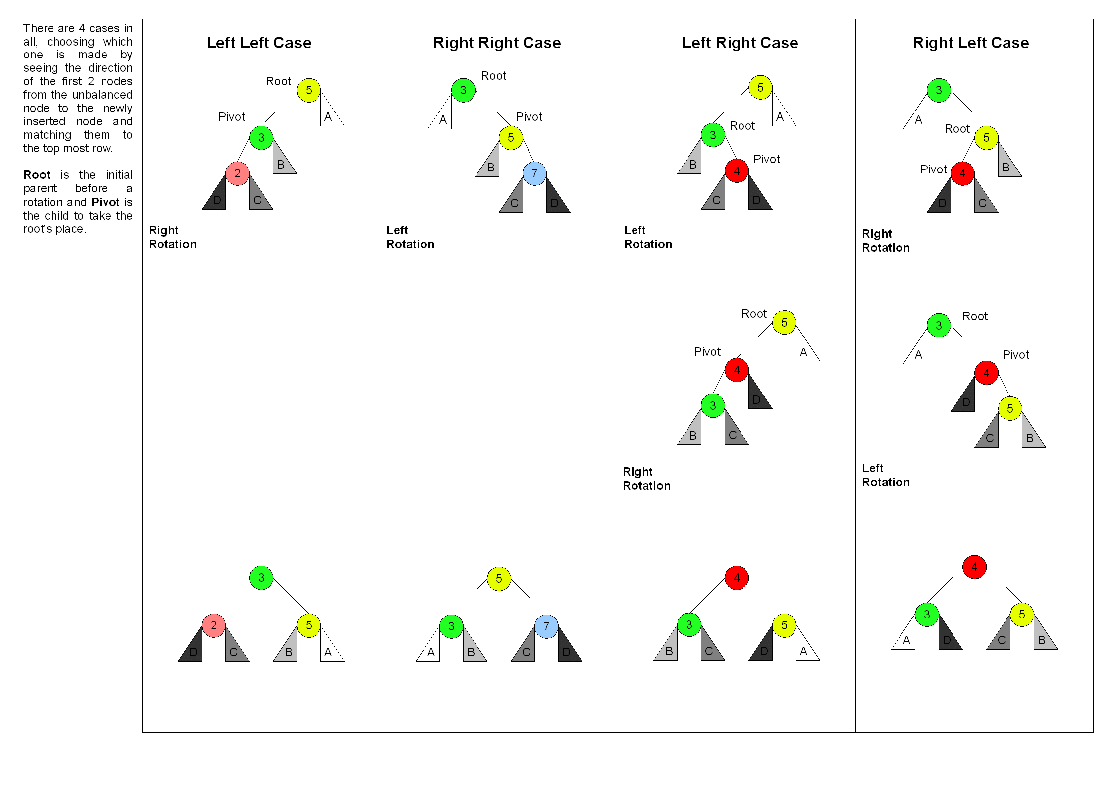
Each repair operation on a “broken” AVL tree takes constant time, $O(1)$.

Are AVL Trees the Best?

Well, it depends! If we’re specifically using AVL trees to model a dictionary, hashmaps (which we’ll cover next semester) offer better performance. However, AVL trees (or modified versions of them) are incredibly versatile and can be used for many tasks:

• Modeling lists with efficient insert, lookup, search, and delete operations.
• Solving a variety of problems that can be represented as tree structures.

Their flexibility makes them a valuable tool for us.

Continue here: 07 Dynamic Programming, Jump Game, Longest Common Subsequence, Edit Distance