08 Gauss Elimination, Elimination Matrices and Solution Sets

Lecture from 11.10.2024 | Video: Videos ETHZ

Computer Vectors and Matrices

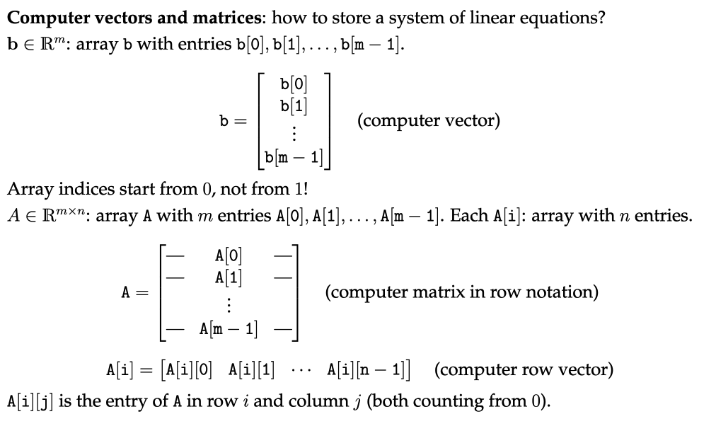
How do we store a system of linear equations $Ax=b$ on a computer? TLDR: We use lists for vectors and lists of lists for matrices.

Gauss Elimination

Gaussian elimination is a systematic method for solving systems of linear equations by performing row operations on an augmented matrix representing the system.

It’s an algorithm for solving $Ax=b$ with quadratic matrices.

The core idea is to systematically transform the augmented matrix $[A|b]$ (representing the system $Ax=b$) into an upper triangular form through row operations.

1. Forward Elimination:

   • Pivot Selection: For each row i, select the first non-zero element in column i as the pivot.
   • Row Normalisation: Divide the i-th row by its pivot element to make the pivot qual to 1. This is called pivot scaling.
   • Elimination: For each row j below row i, subtract a multiple of row i from row j to create zeros below the pivot in column i. The multiplier should be chosen so that the element in position (j, i) becomes zero. This is often denoted by:
     • $R_j\leftarrow R_j-k\cdot R_i$

2. Back Substitution: Once the matrix is upper triangular, we can easily solve for the unknowns. Start with the last equation (which will involve only the last unknown). Solve for this variable, and then substitute it back into the second-to-last equation to solve for the next variable, and so on, until you have solved for all variables. This process is known as back-substitution.

Video:

Elimination Matrices

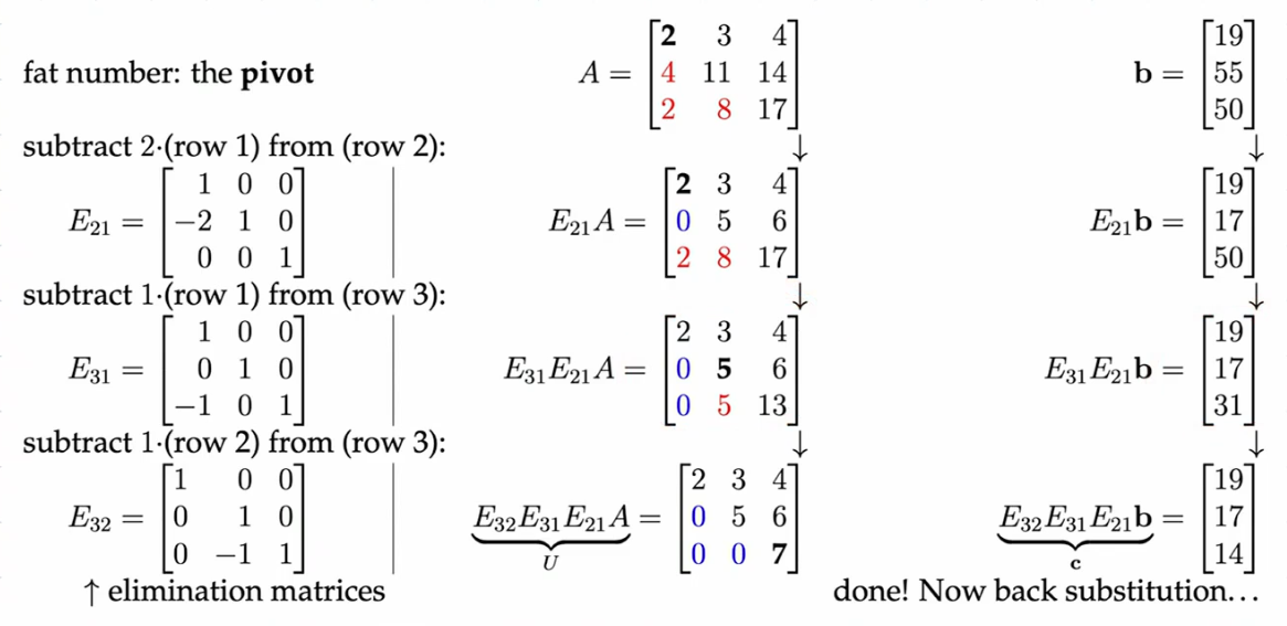
Gaussian elimination can be represented more compactly using elimination matrices. Each row operation corresponds to a specific matrix that, when multiplied with the augmented matrix, performs the desired transformation.

Before diving into elimination matrices, let’s define the elementary row operations:

• Swapping two rows: This operation interchanges the positions of two rows in the matrix.
• Multiplying a row by a non-zero scalar: This operation scales all elements in a row by a constant factor.
• Adding a multiple of one row to another row: This operation involves adding a scaled version of one row to another row, effectively modifying the values in the latter row.

These elementary row operations are crucial for transforming a matrix into an upper triangular form. Importantly, they don’t change the solution to the system of linear equations represented by the matrix. Each operation has a corresponding inverse operation that “undoes” its effect, allowing us to retrieve the original matrix if needed.

Let’s consider the row operation $R_j\leftarrow R_j-k\cdot R_i$. We can represent this operation with an elimination matrix, denoted by $E_{ij}(k)$. This matrix has the following form:

$$E_{ij}(k)=\left[\begin{array}{cccc}1& 0& \dots & 0\\ 0& 1& \dots & 0\\ ⋮& ⋮& \ddots & ⋮\\ 0& -k& \dots & 1\end{array}\right]$$

where the -k is located in the $(j,i)$ position. Multiplying the augmented matrix by $E_{ij}(k)$ effectively performs the row operation described above.

Importantly, we can “undo” these operations. Multiplying the augmented matrix by the inverse of an elimination matrix, denoted by $E_{ij}^{-1}(k)$, will reverse the corresponding row operation. Notice that:

$$E_{ij}^{-1}(k)=E_{ij}(-k)$$

This property allows us to systematically represent Gaussian elimination as a series of matrix multiplications with elimination matrices and their inverses, providing a compact and efficient way to solve systems of linear equations.

General Algorithm

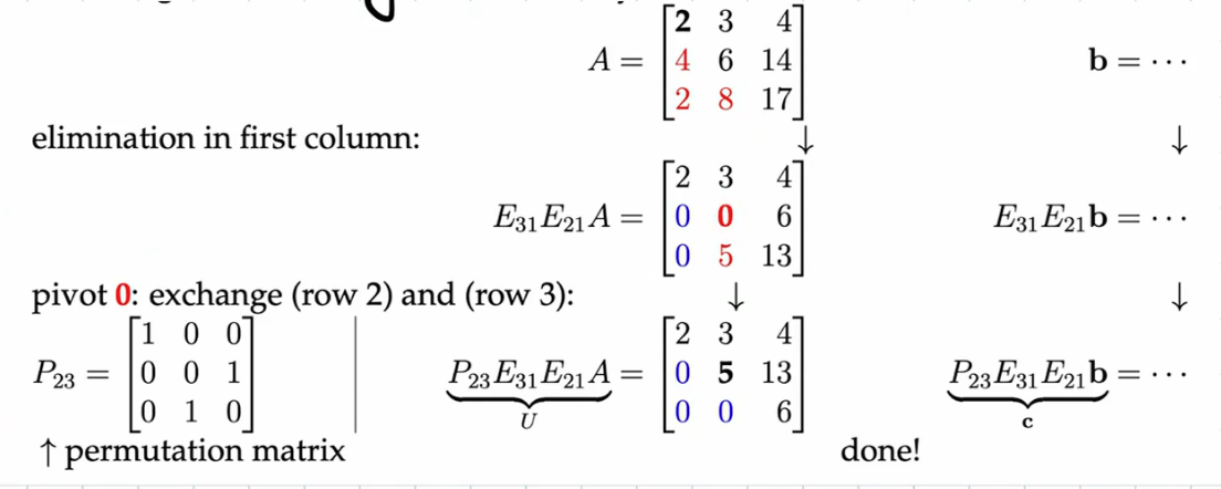
In the case where one of the pivots = 0 → we need to switch rows:

And sometimes it fails (when two pivots are zero and you can’t get rid of them):

Special case where it fails:

$$\left[\begin{array}{ccc}2& 3& 4\\ 0& 5& 6\\ 0& 0& 0\end{array}\right]$$

Solution Possibilities

By carefully observing our resulting (row reduced) matrix, we can glean valuable information about whether a system has:

• A Unique Solution:

  • During elimination: You reach an upper triangular matrix (U) with no zero pivots on the diagonal. Each equation in this form directly corresponds to solving for one variable. This implies a unique solution exists. The values you obtain during back-substitution are your definitive answers.

• Infinitely Many Solutions:

  • During elimination: You encounter at least one row of all zeros (the system becomes dependent). This means there’s redundancy in the equations, allowing for infinitely many combinations of variables that satisfy the system.
  • Interpretation: You can express solutions in terms of free variables —variables that can take on any value, while others are determined by those free variables.

• No Solution (Inconsistent System):

  • During elimination: You encounter a row like this: [0 0 ... 0 | b] where b is non-zero This signifies that the system has a contradiction. The last equation implies something impossible.

Key Points:

• Zero Pivots: Zero pivots are crucial indicators! They often signal redundancy or inconsistency in your system of equations.
• Row Echelon Form: While Gaussian elimination aims for upper triangular form, reaching row echelon form (leading 1s, zeros below leading 1s) is sufficient to determine solution types.

Continue here: 09 Elementary Row Operations, Gauss Elimination, Inverse Matrices, Inverse Theorem