14 Fundamental Subspaces, Column Space, Row Space, Nullspace

Lecture from 01.11.2024 | Video: Videos ETHZ

Fundamental Subspaces of a Matrix

In linear algebra, we often work with matrices and the vector spaces associated with them. A key concept is that of a subspace, which is a subset of a vector space closed under vector addition and scalar multiplication. We can fully characterize a vector space by identifying its basis.

The four fundamental subspaces associated with a matrix $A\in {\mathbb{R}}^{m\times n}$:

1. Column Space ($C(A)$): The column space of $A$, denoted $C(A)$, is the subspace of ${\mathbb{R}}^m$ spanned by the columns of $A$. In other words, $C(A)$ consists of all linear combinations of the columns of $A$.

2. Row Space ($R(A)$): The row space of $A$, denoted $R(A)$, is the subspace of ${\mathbb{R}}^n$ spanned by the rows of $A$. Equivalently, it is the column space of $A^T$ (the transpose of $A$).

3. Null Space ($N(A)$): The null space of $A$, denoted $N(A)$, is the subspace of ${\mathbb{R}}^n$ consisting of all vectors $\mathbf{x}$ that satisfy the homogeneous equation $A\mathbf{x}=0$. The null space represents the set of all inputs to the linear transformation represented by $A$ that produce the zero vector as output.

4. Left Null Space ($N(A^T)$): The left null space of $A$, denoted $N(A^T)$, is the null space of $A^T$. It is a subspace of ${\mathbb{R}}^m$. The left null space can be interpreted as the set of all vectors orthogonal to the column space of $A$. This means that for any $\mathbf{y}\in N(A^T)$ and any $\mathbf{b}\in C(A)$, their dot product is zero: $\mathbf{y}\cdot \mathbf{b}=0$. (Note we will not look at this)

We already have a tool with which we can calculate the basis for all of these subspaces: Gauss-Jordan-Elimination. Recall Gauss-Jordan-Elimination (see Gauss-Jordan Elimination for more):

Column Space

The column space of $A$, denoted $C(A)$, is formally defined as:

$C(A)=\{\mathbf{b}\in {\mathbb{R}}^m|\mathbf{b}=A\mathbf{x}\text{ for some }\mathbf{x}\in {\mathbb{R}}^n\}.$

It represents the set of all possible linear combinations of the columns of $A$, and thus all possible outputs of the linear transformation represented by $A$.

Finding a Basis for $C(A)$ using Gauss-Jordan Elimination:

1. Reduce $A$ to Reduced Row Echelon Form (RREF): Perform Gauss-Jordan elimination on matrix $A$ to obtain its RREF, denoted $R$.
2. Identify Pivot Columns: The pivot columns in $R$ correspond to the linearly independent columns of $A$. The indices of these pivot columns are crucial.
3. Extract Original Columns: The corresponding columns in the original matrix $A$ (not the RREF matrix $R$) form a basis for $C(A)$.

Theorem: Let $A$ be an $m\times n$ matrix, and let $R$ be the RREF of $A$ with pivot column indices $j_1,j_2,\dots ,j_r$. Then the columns $A_{j_1},A_{j_2},\dots ,A_{j_r}$ form a basis for $C(A)$, and $\text{dim}(C(A))=r=\text{rank}(A)$.

Example: Suppose $A=\left[\begin{array}{cccc}1& 2& 0& 3\\ 2& 4& 1& 4\\ 3& 6& 2& 5\end{array}\right]$ After Gauss-Jordan elimination, we obtain the RREF: $R=\left[\begin{array}{cccc}1& 2& 0& 3\\ 0& 0& 1& -2\\ 0& 0& 0& 0\end{array}\right]$

The pivot columns are the first and third columns ($j_1=1$, $j_2=3$). Therefore, the first and third columns of the original matrix $A$ form a basis for $C(A)$: $\text{Basis for }C(A)=\left\{\left[\begin{array}{c}1\\ 2\\ 3\end{array}\right],\left[\begin{array}{c}0\\ 1\\ 2\end{array}\right]\right\}$ The dimension of the column space is 2, which is also the rank of the matrix $A$.

Proof: The independent columns of $A$ are a basis for $C(A)$ and we get these independent columns by doing Gauss-Jordan.

Row Space

The row space of $A$, denoted $R(A)$, is the subspace of ${\mathbb{R}}^n$ spanned by the rows of $A$. It is equivalent to the column space of the transpose of $A$: $R(A)=C(A^T)$.

Finding a Basis for $R(A)$ using Gauss-Jordan Elimination:

1. Reduce $A$ to RREF: Perform Gauss-Jordan elimination on matrix $A$ to obtain its RREF, denoted $R$.
2. Non-zero Rows form a Basis: The non-zero rows of $R$ form a basis for $R(A)$.

Theorem: Let $A$ be an $m\times n$ matrix, and let $R$ be the RREF of $A$. The non-zero rows of $R$ form a basis for $R(A)$, and $\text{dim}(R(A))=r=\text{rank}(A)$.

Important Note: While the column space basis comes from the original matrix $A$, the row space basis comes from the RREF matrix $R$.

Example: Using the same matrix $A$ as in the column space example: $A=\left[\begin{array}{cccc}1& 2& 0& 3\\ 2& 4& 1& 4\\ 3& 6& 2& 5\end{array}\right]$ and its RREF: $R=\left[\begin{array}{cccc}1& 2& 0& 3\\ 0& 0& 1& -2\\ 0& 0& 0& 0\end{array}\right]$ The non-zero rows of $R$ form a basis for $R(A)$:

$\text{Basis for }R(A)=\left\{\left[\begin{array}{cccc}1& 2& 0& 3\end{array}\right],\left[\begin{array}{cccc}0& 0& 1& -2\end{array}\right]\right\}$ The dimension of the row space is 2, which is also the rank of $A$. Note that although $\text{dim}(C(A))=\text{dim}(R(A))$, the basis vectors for $C(A)$ and $R(A)$ are different and belong to different vector spaces (${\mathbb{R}}^m$ and ${\mathbb{R}}^n$ respectively).

Key Takeaway: Row operations preserve the row space but not the column space. The RREF simplifies the process of finding a basis for the row space.

Invariance of Row Space under Multiplication by an Invertible Matrix

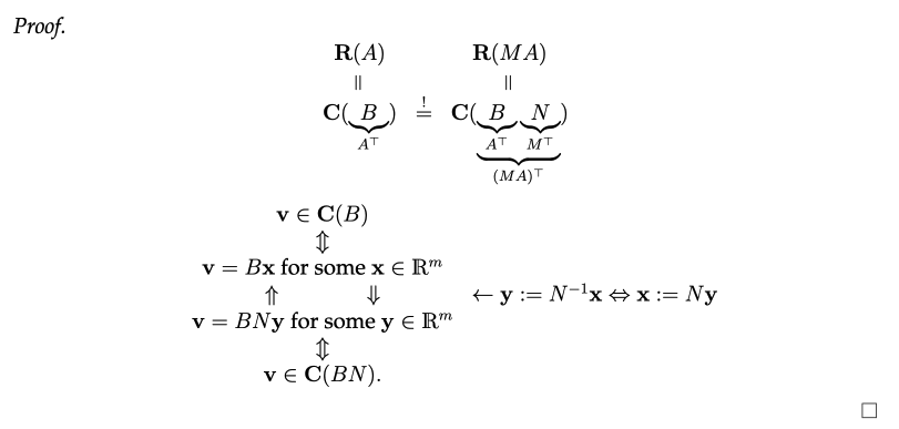
Lemma 4.27: Let $A$ be an $m\times n$ matrix, and let $M$ be an invertible $m\times m$ matrix. Then $R(A)=R(MA)$.

This lemma states that multiplying a matrix $A$ by an invertible matrix $M$ on the left does not change its row space.

Proof

The core idea is to understand the connection between row spaces and column spaces through transposes:

• Row space is the column space of the transpose: $R(A)=C(A^T)$.

We’ll use the following notation:

• $B=A^T$ (transpose of $A$)
• $N=M^T$ (transpose of $M$)

The proof revolves around showing that $C(B)=C(BN)$:

1. Start with the row space of A: Consider any vector $\mathbf{v}$ in the row space of $A$ ($R(A)$): $\mathbf{v}\in R(A)$
2. Express it as a column space vector: Since $R(A)=C(A^T)=C(B)$, we can express $\mathbf{v}$ as a linear combination of the columns of $B$: $\mathbf{v}=B\mathbf{x}\text{ for some }\mathbf{x}\in {\mathbb{R}}^m$
3. Introduce M and relate to the row space of MA: To connect to the row space of $MA$, we introduce the invertible matrix $M$. Since $M$ is invertible, its inverse $N^{-1}$ exists. Let’s introduce a new vector $\mathbf{y}$ related to $\mathbf{x}$ by the equation $\mathbf{y}=N^{-1}\mathbf{x}$.

This means $\mathbf{x}=N\mathbf{y}$ (multiplying both sides by $N$). Now, we can rewrite $\mathbf{v}$ in terms of $\mathbf{y}$: $\mathbf{v}=B\mathbf{x}=B(N\mathbf{y})=(BN)\mathbf{y}$ 4. Show v is in the column space of BN: Since $\mathbf{v}$ is a linear combination of the columns of $BN$, it belongs to the column space of $BN$:

$\mathbf{v}\in C(BN)$

1. Connecting to the row space of MA: Recall that $C(BN)=C((MA{)}^T)$ because the transpose of a product is the product of the transposes in reverse order. Therefore, $C(BN)$ is the row space of $MA$: $C(BN)=C((MA{)}^T)=R(MA)$
2. Equivalence: By following these steps, we’ve shown that:
   • If $\mathbf{v}$ is in $R(A)$, then it’s also in $R(MA)$. This implies $R(A)\subseteq R(MA)$.
   • Since $M$ is invertible, we can repeat the same logic using $M^{-1}$ to show that $R(MA)\subseteq R(A)$.
   • Combining both directions, we conclude that $R(A)=R(MA)$.

Finding a Basis for $R(A)$ using REF

Theorem 4.28: Let $A$ be an $m\times n$ matrix, and let $R$ be the REF of $A$ with pivot column indices $j_1,j_2,\dots ,j_r$. Then the first $r$ rows of $R$ form a basis for the row space $R(A)$, and $\text{dim}(R(A))=r=\text{rank}(A)$.

Why This Works:

The theorem builds on the understanding of row operations, REF structure, and the connection between row spaces and column spaces through transposes. Let’s break down the key reasons why this theorem holds true:

1. Row Operations Preserve Row Space: Gauss-Jordan elimination, which produces the REF, involves row operations. We already know from Lemma 4.27 (see Invariance of Row Space under Multiplication by an Invertible Matrix) that row operations (equivalent to multiplication by invertible matrices) don’t change the row space. Therefore, $R(A)=R(R)$.
2. Structure of RREF: The REF $R$ has the following key properties:

• Pivot Rows: The first $r$ rows of $R$ are the non-zero rows, where $r$ is the rank of $A$.
• Zero Rows: The remaining $m-r$ rows are all zero.

3. Linear Independence: The first $r$ rows of $R$ are linearly independent. This is because each row has a pivot position (leading 1) in a column that is unique to that row. No row can be expressed as a linear combination of the other rows.
4. Spanning: The first $r$ rows of $R$ span the entire row space $R(R)$. This is because any linear combination of the original rows of $A$ can be rewritten as a linear combination of the rows of $R$, thanks to the row operations.

By using row operations to put $A$ in REF, we achieve two things:

• We obtain a set of linearly independent vectors (the non-zero rows of $R$).
• These vectors span the entire row space $R(A)$.

Therefore, these vectors form a basis for the row space of $A$.

Proof

Let $R_0$ be the result of Gauss-Jordan elimination on $A$. We know that $R_0=MA$, where $M$ is a product of elementary matrices (invertible). By Lemma 4.27, $R(A)=R(R_0)$.

The first $r$ rows of $R_0$ are the non-zero rows of $R_0$. These rows are linearly independent because each row has a pivot position (leading 1) in a column that is unique to that row. This implies that no row can be expressed as a linear combination of the other rows.

We now show that the first $r$ rows of $R_0$ span $R(A)$. Let $\mathbf{v}\in R(A)$. Since $R(A)=R(R_0)$, we can write $\mathbf{v}$ as a linear combination of the rows of $R_0$. Let $\mathbf{u}$ be a vector containing the coefficients of this linear combination. Then, $\mathbf{v}={\mathbf{u}}^T{R}_0$.

Since the first $r$ rows of $R_0$ are linearly independent, the remaining $m-r$ rows must be linear combinations of the first $r$ rows. Thus, we can rewrite $\mathbf{v}$ as a linear combination of only the first $r$ rows of $R_0$.

This shows that the first $r$ rows of $R_0$ span $R(A)$. Since they are also linearly independent, they form a basis for $R(A)$.

Since $R_0=MA$, we can conclude that the first $r$ rows of $R$ (which are the same as the first $r$ rows of $R_0$) form a basis for $R(A)$.

Example:

Consider the matrix $A$ and its REF from previous examples:

$A=\left[\begin{array}{cccc}1& 2& 0& 3\\ 2& 4& 1& 4\\ 3& 6& 2& 5\end{array}\right]\Rightarrow R=\left[\begin{array}{cccc}1& 2& 0& 3\\ 0& 0& 1& -2\\ 0& 0& 0& 0\end{array}\right]$

The first two rows of $R$ form a basis for $R(A)$:

$\text{Basis for }R(A)=\left\{\left[\begin{array}{cccc}1& 2& 0& 3\end{array}\right],\left[\begin{array}{cccc}0& 0& 1& -2\end{array}\right]\right\}$

We can conclude that $\text{dim}(R(A))=2$ and the rank of $A$ is 2.

Observation: $\text{Because }\underset{\text{rank}(A)}{\underbrace{\dim (\mathbf{C}(A))}}=\underset{\text{Theorem 4.28}}{\underbrace{\dim (\mathbf{R}(A))}}=\underset{\text{Def. of row space}}{\underbrace{\stackrel{\text{rank}(A^{\top )}}{\overbrace{\dim (\mathbf{C}(A^{\top }))}}}},\text{row rank equals column rank}$

Row Rank Equals Column Rank

Theorem 4.29: Let $A$ be an $m\times n$ matrix. Then $\text{rank}(A)=\text{rank}(A^T)$.

Why This Works:

This theorem directly follows from the fact that the dimension of the column space of $A$ equals the dimension of the row space of $A$, which in turn equals the dimension of the column space of $A^T$.

• Dimensionality: We’ve established that $\text{dim}(C(A))=\text{rank}(A)$ and $\text{dim}(R(A))=\text{rank}(A)$.
• Transpose Relationship: We also know that $R(A)=C(A^T)$.

Putting these together, we have:

• $\text{rank}(A)=\text{dim}(C(A))$
• $\text{rank}(A)=\text{dim}(R(A))=\text{dim}(C(A^T))=\text{rank}(A^T)$

Therefore, the row rank of a matrix is always equal to its column rank.

This is a fundamental result in linear algebra, emphasizing the close relationship between row space and column space.

Nullspace $N(A)$

The nullspace (also called kernel) of a matrix $A\in {\mathbb{R}}^{m\times n}$, denoted $N(A)$, is the set of all vectors $\mathbf{x}\in {\mathbb{R}}^n$ that satisfy the homogeneous equation $A\mathbf{x}=0$. Formally:

$N(A)=\{\mathbf{x}\in {\mathbb{R}}^n|A\mathbf{x}=0\}$

Key Properties and Interpretations

• Subspace: $N(A)$ is a subspace of ${\mathbb{R}}^n$. This can be easily verified by checking closure under addition and scalar multiplication.
• Solutions to Homogeneous System: The nullspace represents all solutions to the homogeneous system of linear equations represented by $A\mathbf{x}=0$.
• Kernel of Linear Transformation: If $A$ represents a linear transformation, $N(A)$ is the kernel of that transformation – the set of all vectors that map to the zero vector.

Invertible Matrices and Nullspace

Lemma 4.33: Let $A$ be an $m\times n$ matrix, and $M$ be an invertible $m\times m$ matrix. Then $N(A)=N(MA)$.

This lemma states that multiplying a matrix $A$ by an invertible matrix $M$ on the left does not change its nullspace.

Proof:

We need to show that any vector in $N(A)$ is also in $N(MA)$, and vice-versa.

1. Suppose $x\in N(A)$: This means $A\mathbf{x}=0$. Now consider $(MA)\mathbf{x}=M(A\mathbf{x})=M0=0$. Therefore, $\mathbf{x}$ is also in $N(MA)$. This shows $N(A)\subseteq N(MA)$.
2. Suppose $x\in N(MA)$: This means $(MA)\mathbf{x}=0$. Since $M$ is invertible, we can multiply both sides by $M^{-1}$: $M^{-1}(MA)\mathbf{x}=M^{-1}0$, which simplifies to $A\mathbf{x}=0$. Thus, $\mathbf{x}$ is also in $N(A)$. This shows $N(MA)\subseteq N(A)$.

Since $N(A)\subseteq N(MA)$ and $N(MA)\subseteq N(A)$, we conclude that $N(A)=N(MA)$.

This lemma is crucial for understanding why we can use the RREF of $A$ to find the nullspace of $A$. The RREF is obtained by multiplying $A$ by a series of invertible elementary matrices. Thus, the nullspace of $A$ is the same as the nullspace of its RREF, which is much easier to compute.

Finding a Basis for $N(A)$ using Gauss-Jordan Elimination

Theorem 4.35:

1. Reduce A to REF: Perform Gauss-Jordan elimination on $A$ to obtain its REF, denoted $R$.
2. Identify Free and Basic Variables: In the REF, identify the pivot columns and the corresponding basic variables. The remaining variables are the free variables.
3. Express Basic Variables in terms of Free Variables: Express each basic variable as a linear combination of the free variables, based on the equations represented by the rows of $R$.
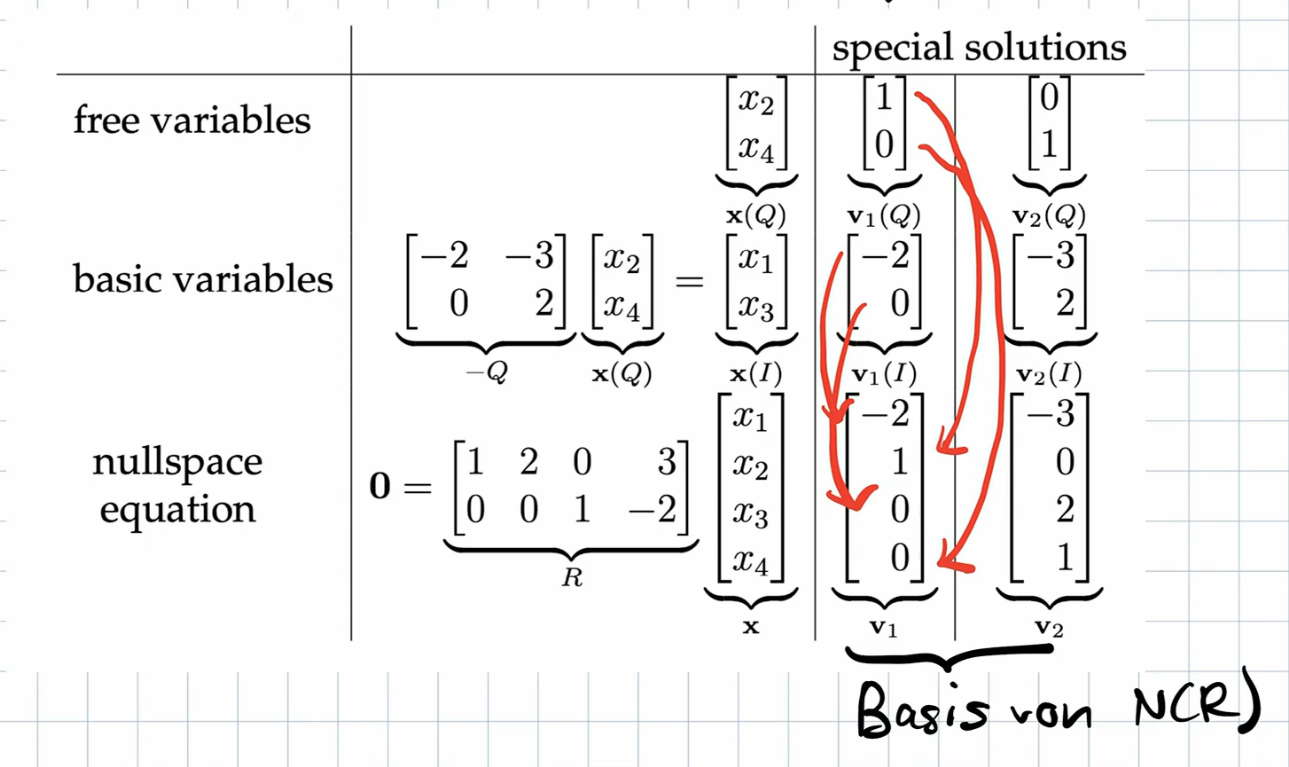
4. Form Special Solutions: For each free variable, create a special solution by setting that free variable to 1 and all other free variables to 0. Then, solve for the basic variables using the expressions derived in the previous step.
5. Special Solutions Form a Basis: The set of special solutions forms a basis for $N(A)$.

Example

Let’s revisit our example matrix $A$ and its REF $R$:

$A=\left[\begin{array}{cccc}1& 2& 0& 3\\ 2& 4& 1& 4\\ 3& 6& 2& 5\end{array}\right]\Rightarrow R=\left[\begin{array}{cccc}1& 2& 0& 3\\ 0& 0& 1& -2\\ 0& 0& 0& 0\end{array}\right]$

• Basic and Free Variables: The pivot columns are 1 and 3, so $x_1$ and $x_3$ are basic variables. $x_2$ and $x_4$ are free variables.

• Express Basic in terms of Free: From the REF, we have the equations:

  Notice how we can choose our free variables $x(Q)$ and then read of $x(I)$.

• Special Solutions:

• Setting $x_2=1$ and $x_4=0$, we get $x_1=-2$ and $x_3=0$. This gives the special solution ${\mathbf{v}}_1=\left[\begin{array}{c}-2\\ 1\\ 0\\ 0\end{array}\right]$.

• Setting $x_2=0$ and $x_4=1$, we get $x_1=-3$ and $x_3=2$. This gives the special solution ${\mathbf{v}}_2=\left[\begin{array}{c}-3\\ 0\\ 2\\ 1\end{array}\right]$.

• Basis for N(A): The basis for the nullspace is $\{{\mathbf{v}}_1,{\mathbf{v}}_2\}$.

Therefore, $\text{dim}(N(A))=2$, which is $n-r$ (number of columns minus the rank).

The Solution Space of $A\mathbf{x}=\mathbf{b}$

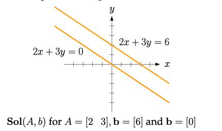
Definition 4.39: For a matrix $A\in {\mathbb{R}}^{m\times n}$ and a vector $\mathbf{b}\in {\mathbb{R}}^m$, the solution space (or solution set) of the linear system $A\mathbf{x}=\mathbf{b}$ is defined as: $\text{Sol}(A,\mathbf{b})=\{\mathbf{x}\in {\mathbb{R}}^n|A\mathbf{x}=\mathbf{b}\}$ This set contains all vectors $\mathbf{x}$ that satisfy the given linear system.

Key Properties and Considerations

• Subspace (only if b = 0): $\text{Sol}(A,\mathbf{b})$ is a subspace of ${\mathbb{R}}^n$ if and only if $\mathbf{b}=0$. If $\mathbf{b}\ne 0$, then $\text{Sol}(A,\mathbf{b})$ is not a subspace because it doesn’t contain the zero vector (since $A0=0\ne \mathbf{b}$).
• Affine Subspace (if b ≠ 0): When $\mathbf{b}\ne 0$, and a solution exists, $\text{Sol}(A,\mathbf{b})$ is called an affine subspace. It can be thought of as a subspace that has been “shifted” or “translated” away from the origin.
• Existence of Solutions: The solution space might be empty (i.e., no solutions exist) if $\mathbf{b}$ is not in the column space of $A$.
• Relationship to Nullspace: The solution space is closely related to the nullspace of $A$. Theorem 4.40 formalizes this relationship.

Structure of the Solution Space

Theorem 4.40: Let $A$ be an $m\times n$ matrix, and $\mathbf{b}\in {\mathbb{R}}^m$. Let ${\mathbf{x}}_p$ be a particular solution of $A\mathbf{x}=\mathbf{b}$ (if one exists). Then: $\text{Sol}(A,\mathbf{b})=\{{\mathbf{x}}_p+\mathbf{v}|\mathbf{v}\in N(A)\}$ This theorem states that the solution space consists of all vectors obtained by adding a particular solution ${\mathbf{x}}_p$ to every vector in the nullspace of $A$.

Proof:

We need to show that any vector in $\text{Sol}(A,\mathbf{b})$ can be written in the form ${\mathbf{x}}_p+\mathbf{v}$, where $\mathbf{v}\in N(A)$, and vice-versa.

1. Let $\mathbf{y}\in \text{Sol}(A,\mathbf{b})$: This means $A\mathbf{y}=\mathbf{b}$. Since ${\mathbf{x}}_p$ is also a solution, $A{\mathbf{x}}_p=\mathbf{b}$. Subtracting these equations gives: $A\mathbf{y}-A{\mathbf{x}}_p=\mathbf{b}-\mathbf{b}$ $A(\mathbf{y}-{\mathbf{x}}_p)=0$ This means $\mathbf{y}-{\mathbf{x}}_p$ is in the nullspace of $A$. Let $\mathbf{v}=\mathbf{y}-{\mathbf{x}}_p$. Then $\mathbf{v}\in N(A)$, and $\mathbf{y}={\mathbf{x}}_p+\mathbf{v}$. So, any solution $\mathbf{y}$ can be written in the desired form.

2. Let $\mathbf{x}={\mathbf{x}}_p+\mathbf{v}$, where $\mathbf{v}\in N(A)$: This means $A\mathbf{v}=0$. Now, let’s check if $\mathbf{x}$ is a solution to $A\mathbf{x}=\mathbf{b}$: $A\mathbf{x}=A({\mathbf{x}}_p+\mathbf{v})=A{\mathbf{x}}_p+A\mathbf{v}=\mathbf{b}+0=\mathbf{b}$ Thus, $\mathbf{x}$ is indeed a solution, so $\mathbf{x}\in \text{Sol}(A,\mathbf{b})$.

This proves that the solution set has the structure described in the theorem. If a particular solution exists, every other solution can be obtained by adding a vector from the nullspace to that particular solution. This highlights the fundamental relationship between the solution space of a non-homogeneous system and the nullspace of the corresponding matrix.

Intuition:

• ${\mathbf{x}}_p$: This represents one specific way to reach $\mathbf{b}$ through the transformation defined by $A$.
• $N(A)$: The nullspace captures all the directions along which you can move without changing the result (i.e., $A\mathbf{v}=0$ for $\mathbf{v}\in N(A)$).
• ${\mathbf{x}}_p+\mathbf{v}$: Adding vectors from the nullspace to the particular solution finds all other solutions. These represent variations of the particular solution that don’t affect the target $\mathbf{b}$.

Dimensions and Structure of Solution Spaces

1. Dimensionality of $Sol(A,b)$: When $\text{Sol}(A,\mathbf{b})$ has a solution (i.e., the system $A\mathbf{x}=\mathbf{b}$ is consistent), it has a “dimension” of $n-r$, where $r$ is the rank of $A$ and $n$ is the number of columns in $A$. This dimension intuitively represents the number of “degrees of freedom” in the solution space.

2. Parallelism to $N(A)$: The solution space $\text{Sol}(A,\mathbf{b})$ can be viewed as a parallel translation of the nullspace $N(A)$. Imagine the nullspace as a subspace (or a “plane” in higher dimensions) passing through the origin. The solution space is obtained by shifting this “plane” by the particular solution ${\mathbf{x}}_p$.

3. Cases Based on $Rank(r)$:

• $r=m$ (Full Rank): If the rank of $A$ equals the number of rows ($r=m$), then the RREF of $A$ will have no rows full of zeros. This means that the system $R_0\mathbf{x}=\mathbf{c}$ (where $R_0$ is the RREF of $A$ and $\mathbf{c}$ is obtained from $\mathbf{b}$ through the same row operations) will always have a solution. Consequently, the original system $A\mathbf{x}=\mathbf{b}$ will also have a solution. In this case, the solution space is non-empty, and its dimension is $n-r=n-m$, which could be 0 or greater. If it is 0, there is only one solution.

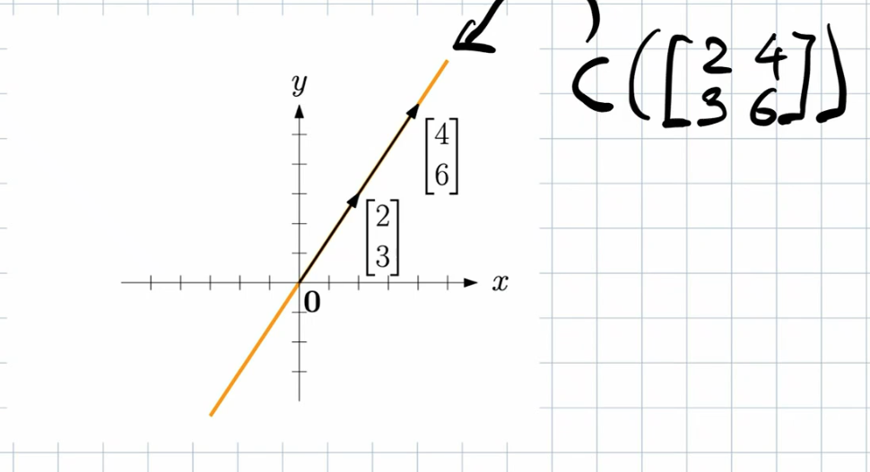
• $r<m$ (Rank Deficiency): When the rank of $A$ is less than the number of rows ($r<m$), this means the column space $C(A)$ has a lower dimension than the space it’s embedded in (${\mathbb{R}}^m$). Imagine $C(A)$ as a “plane” (or a “line” in a 3D space) within a higher-dimensional space. Since $C(A)$ is “smaller” than the space it occupies, there will be many vectors $\mathbf{b}$ that lie outside of this “plane”. For these vectors $\mathbf{b}$, there’s no way to express $\mathbf{b}$ as a linear combination of the columns of $A$, meaning there’s no solution to the system $A\mathbf{x}=\mathbf{b}$.

Example: Rank Deficiency

Continue here: 15 Orthogonal Vectors and Orthogonal Complements of Subspaces